Zero-point renormalization of the band gap and temperature-dependent band gaps with GWPT
This tutorial is similar to eph4zpr. Also in this lesson, we compute the electron self-energy due to phonons, obtain the zero-point renormalization (ZPR) of the band gap and temperature-dependent band energies within the harmonic approximation. The main difference with respect to eph4zpr, is that, in this lesson, the e-ph matrix elements are computed within the GWPT formalism [Li2019].
It is assumed that the user has already completed the two tutorials RF1 and RF2, and that they are familiar with the calculation of ground state (GS) and response properties, in particular phonons, Born effective charges (BECs) and the high-frequency dielectric tensor.
The user should have read the introduction tutorial for the EPH code, and (very important) the description of the gstore-based approach, before running these examples.
Also, you are kindly invited to read the first GW tutorial if you are not familiar with the GW implementation in Abinit. A brief description of the formalism and of the equations implemented in the code can be found in the GW_notes.
Note that in this tutorial, we will be using the conventional GW implementation in Fourier space and frequency-domain with quartic scaling with the number of atoms. A more efficient algorithm with cubic scaling is provided by the GWR code described in the GWR1 tutorial. Unfortunately, at the time of writing, the GWR code is not yet interfaced with GWPT.
This lesson should take about 2.0 hours.
Formalism
In the GWPT method [Li2019], the e-ph matrix elements are computed by replacing the first-order change of the KS Hamiltonian induced by a phonon with the variation of the \(GW\) self-energy:
with
and \(\widetilde{W}\) is the frequency convolution of the screened Coulomb interaction:
Besides the summations over empty states \(n'\), the equation requires the knowledge of the screened interaction \(W\) as well as the (full) first-order derivative of the KS states \(\partial_{\kappa\alpha\mathbf{q}} \psi_{n^{\prime}}\) induced by an atomic displacement of atom \(\kappa\) along direction \(\alpha\) modulated by the wavevector \(\mathbf{q}\). Both terms can be computed by Abinit.
The screened interaction \(W\) is computed in terms of a sum of states with optdriver 3, and the results are stored in the SCR file. The first-order derivative of the KS states, on the contrary, is computed on the fly by the GWPT subdriver by solving a non-self-consistent (NSCF) Sternheimer equation as explained in the sections below.
Warning
Please note that ZPR computations at the GWPT level are still a field of active research, especially in polar materials where additional long-range (LR) terms of many-body nature appear in the e-ph matrix elements. In this tutorial, we won’t be able to converge the calculation; hence, we mainly focus on explaining the different steps involved and the input parameters affecting the quality of the calculation and the predictive power. Hopefully, additional techniques and algorithmic improvements will be made available in forthcoming Abinit versions in order to accelerate GWPT calculations without spoiling accuracy (stay tuned).
Getting started
Note
Supposing you made your own installation of ABINIT, the input files to run the examples are in the ~abinit/tests/ directory where ~abinit is the absolute path of the abinit top-level directory. If you have NOT made your own install, ask your system administrator where to find the package, especially the executable and test files.
In case you work on your own PC or workstation, to make things easier, we suggest you define some handy environment variables by executing the following lines in the terminal:
export ABI_HOME=Replace_with_absolute_path_to_abinit_top_level_dir # Change this line
export PATH=$ABI_HOME/src/98_main/:$PATH      # Do not change this line: path to executable
export ABI_TESTS=$ABI_HOME/tests/             # Do not change this line: path to tests dir
export ABI_PSPDIR=$ABI_TESTS/Pspdir/  # Do not change this line: path to pseudos dir
Examples in this tutorial use these shell variables: copy and paste
the code snippets into the terminal (remember to set ABI_HOME first!) or, alternatively,
source the set_abienv.sh script located in the ~abinit directory:
source ~abinit/set_abienv.sh
The ‘export PATH’ line adds the directory containing the executables to your PATH so that you can invoke the code by simply typing abinit in the terminal instead of providing the absolute path.
To execute the tutorials, create a working directory (Work*) and
copy there the input files of the lesson.
Most of the tutorials do not rely on parallelism (except specific tutorials on parallelism). However you can run most of the tutorial examples in parallel with MPI, see the topic on parallelism.
Before beginning, you might consider working in a different subdirectory as for the other tutorials. Why not create Work_eph4zpr_gwpt in $ABI_TESTS/tutorespfn/Input?
cd $ABI_TESTS/tutorespfn/Input
mkdir Work_eph4zpr_gwpt
cd Work_eph4zpr_gwpt
In this tutorial, we prefer to focus on the use of the GWPT subdriver of the EPH code hence we will be using pre-computed DDB and DFPT POT and DEN files to bypass the DFPT part. We also provide a GS DEN.nc file to initialize the NSCF calculation and a GS POT file with the KS potential required to solve the NSCF Sternheimer equation.
If git is installed on your machine, one can easily fetch the entire repository with:
git clone https://github.com/abinit/MgO_eph_zpr.git
Alternatively, use wget:
wget https://github.com/abinit/MgO_eph_zpr/archive/master.zip
or curl:
curl -L https://github.com/abinit/MgO_eph_zpr/archive/master.zip -o master.zip
or simply copy the tarball by clicking the “download button” available in the github web page, unzip the file and rename the directory with:
unzip master.zip
mv MgO_eph_zpr-master MgO_eph_zpr_gwpt
Warning
The directory with the precomputed files must be located in the same working directory
in which you will be executing the tutorial and must be named MgO_eph_zpr_gwpt.
At this point, copy all the input files for the tutorial with:
cp ../Input/teph4zpr_gwpt_* .
and we are ready to go.
Merging partial DDB, DFPT POT and DEN files
The first steps are similar to the ones used in the eph4zpr tutorial. First, we merge the partial DDB files containing the dynamical matrix evaluated for different \(\mathbf{q}\)-points and atomic perturbations by executing:
mrgddb < teph4zpr_gwpt_1.abi
with the following input file:
teph4zpr_gwpt_1_DDB
MgO phonons on 4x4x4 q-mesh
28
MgO_eph_zpr/flow_zpr_mgo/w1/t3/outdata/out_DDB
MgO_eph_zpr/flow_zpr_mgo/w1/t4/outdata/out_DDB
MgO_eph_zpr/flow_zpr_mgo/w1/t5/outdata/out_DDB
MgO_eph_zpr/flow_zpr_mgo/w1/t6/outdata/out_DDB
MgO_eph_zpr/flow_zpr_mgo/w1/t7/outdata/out_DDB
MgO_eph_zpr/flow_zpr_mgo/w1/t8/outdata/out_DDB
MgO_eph_zpr/flow_zpr_mgo/w1/t9/outdata/out_DDB
MgO_eph_zpr/flow_zpr_mgo/w1/t10/outdata/out_DDB
MgO_eph_zpr/flow_zpr_mgo/w1/t11/outdata/out_DDB
MgO_eph_zpr/flow_zpr_mgo/w1/t12/outdata/out_DDB
MgO_eph_zpr/flow_zpr_mgo/w1/t13/outdata/out_DDB
MgO_eph_zpr/flow_zpr_mgo/w1/t14/outdata/out_DDB
MgO_eph_zpr/flow_zpr_mgo/w1/t15/outdata/out_DDB
MgO_eph_zpr/flow_zpr_mgo/w1/t16/outdata/out_DDB
MgO_eph_zpr/flow_zpr_mgo/w1/t17/outdata/out_DDB
MgO_eph_zpr/flow_zpr_mgo/w1/t18/outdata/out_DDB
MgO_eph_zpr/flow_zpr_mgo/w1/t19/outdata/out_DDB
MgO_eph_zpr/flow_zpr_mgo/w1/t20/outdata/out_DDB
MgO_eph_zpr/flow_zpr_mgo/w1/t21/outdata/out_DDB
MgO_eph_zpr/flow_zpr_mgo/w1/t22/outdata/out_DDB
MgO_eph_zpr/flow_zpr_mgo/w1/t23/outdata/out_DDB
MgO_eph_zpr/flow_zpr_mgo/w1/t24/outdata/out_DDB
MgO_eph_zpr/flow_zpr_mgo/w1/t25/outdata/out_DDB
MgO_eph_zpr/flow_zpr_mgo/w1/t26/outdata/out_DDB
MgO_eph_zpr/flow_zpr_mgo/w1/t27/outdata/out_DDB
MgO_eph_zpr/flow_zpr_mgo/w1/t28/outdata/out_DDB
MgO_eph_zpr/flow_zpr_mgo/w1/t29/outdata/out_DDB
MgO_eph_zpr/flow_zpr_mgo/w1/t30/outdata/out_DDB

##############################################################
# This section is used only for regression testing of ABINIT #
##############################################################
#%%<BEGIN TEST_INFO>
#%% [setup]
#%% executable = mrgddb
#%% test_chain =  teph4zpr_gwpt_1.abi, teph4zpr_gwpt_2.abi, teph4zpr_gwpt_3.abi, teph4zpr_gwpt_4.abi,
#%%               teph4zpr_gwpt_5.abi, teph4zpr_gwpt_6.abi, teph4zpr_gwpt_7.abi, teph4zpr_gwpt_8.abi
#%% exclude_builders = scope_gnu_10.2_paral
#%% [files]
#%% use_git_submodule = MgO_eph_zpr
#%% files_to_test =
#%%   teph4zpr_gwpt_1.stdout, tolnlines= 57, tolabs=  3.000e-02, tolrel=  6.000e-03
#%% [paral_info]
#%% max_nprocs = 1
#%% [extra_info]
#%% authors = M. Giantomassi
#%% keywords = NC, DFPT, EPH, GWPT
#%% description = Merge precomputed DDB files stored in the MgO_eph_zpr git submodule
#%%<END TEST_INFO>
that lists the relative paths of the partial DDB files in the MgO_eph_zpr directory.
Then we merge the DFPT potential with the mrgdv tool using the command.
mrgdv < teph4zpr_gwpt_2.abi
with the following input file:
teph4zpr_gwpt_2_DVDB
28
MgO_eph_zpr/flow_zpr_mgo/w1/t3/outdata/out_POT1.nc
MgO_eph_zpr/flow_zpr_mgo/w1/t4/outdata/out_POT4.nc
MgO_eph_zpr/flow_zpr_mgo/w1/t5/outdata/out_POT1.nc
MgO_eph_zpr/flow_zpr_mgo/w1/t6/outdata/out_POT2.nc
MgO_eph_zpr/flow_zpr_mgo/w1/t7/outdata/out_POT4.nc
MgO_eph_zpr/flow_zpr_mgo/w1/t8/outdata/out_POT5.nc
MgO_eph_zpr/flow_zpr_mgo/w1/t9/outdata/out_POT1.nc
MgO_eph_zpr/flow_zpr_mgo/w1/t10/outdata/out_POT2.nc
MgO_eph_zpr/flow_zpr_mgo/w1/t11/outdata/out_POT4.nc
MgO_eph_zpr/flow_zpr_mgo/w1/t12/outdata/out_POT5.nc
MgO_eph_zpr/flow_zpr_mgo/w1/t13/outdata/out_POT1.nc
MgO_eph_zpr/flow_zpr_mgo/w1/t14/outdata/out_POT4.nc
MgO_eph_zpr/flow_zpr_mgo/w1/t15/outdata/out_POT1.nc
MgO_eph_zpr/flow_zpr_mgo/w1/t16/outdata/out_POT2.nc
MgO_eph_zpr/flow_zpr_mgo/w1/t17/outdata/out_POT3.nc
MgO_eph_zpr/flow_zpr_mgo/w1/t18/outdata/out_POT4.nc
MgO_eph_zpr/flow_zpr_mgo/w1/t19/outdata/out_POT5.nc
MgO_eph_zpr/flow_zpr_mgo/w1/t20/outdata/out_POT6.nc
MgO_eph_zpr/flow_zpr_mgo/w1/t21/outdata/out_POT1.nc
MgO_eph_zpr/flow_zpr_mgo/w1/t22/outdata/out_POT3.nc
MgO_eph_zpr/flow_zpr_mgo/w1/t23/outdata/out_POT4.nc
MgO_eph_zpr/flow_zpr_mgo/w1/t24/outdata/out_POT6.nc
MgO_eph_zpr/flow_zpr_mgo/w1/t25/outdata/out_POT1.nc
MgO_eph_zpr/flow_zpr_mgo/w1/t26/outdata/out_POT4.nc
MgO_eph_zpr/flow_zpr_mgo/w1/t27/outdata/out_POT1.nc
MgO_eph_zpr/flow_zpr_mgo/w1/t28/outdata/out_POT2.nc
MgO_eph_zpr/flow_zpr_mgo/w1/t29/outdata/out_POT4.nc
MgO_eph_zpr/flow_zpr_mgo/w1/t30/outdata/out_POT5.nc

##############################################################
# This section is used only for regression testing of ABINIT #
##############################################################
#%%<BEGIN TEST_INFO>
#%% [setup]
#%% executable = mrgdv
#%% test_chain =  teph4zpr_gwpt_1.abi, teph4zpr_gwpt_2.abi, teph4zpr_gwpt_3.abi, teph4zpr_gwpt_4.abi,
#%%               teph4zpr_gwpt_5.abi, teph4zpr_gwpt_6.abi, teph4zpr_gwpt_7.abi, teph4zpr_gwpt_8.abi
#%% exclude_builders = scope_gnu_10.2_paral
#%% [files]
#%% use_git_submodule = MgO_eph_zpr
#%% files_to_test =
#%%   teph4zpr_gwpt_2.stdout, tolnlines= 57, tolabs=  3.000e-02, tolrel=  6.000e-03
#%% [paral_info]
#%% max_nprocs = 1
#%% [extra_info]
#%% authors = M. Giantomassi
#%% keywords = NC, DFPT, EPH, GWPT
#%% description = Merge precomputed DFPT POT files stored in the MgO_eph_zpr git submodule
#%%<END TEST_INFO>
that lists the relative paths of the partial DFPT POT files in the MgO_eph_zpr directory.
Note that, in the case of GWPT, we also need to merge the files with the first-order derivatives of the density, as the GWPT code needs to compute:
This is done by executing
mrgdv < teph4zpr_gwpt_3.abi
with the following input file:
teph4zpr_gwpt_3_DRHODB
28
MgO_eph_zpr/flow_zpr_mgo/w1/t3/outdata/out_DEN1.nc
MgO_eph_zpr/flow_zpr_mgo/w1/t4/outdata/out_DEN4.nc
MgO_eph_zpr/flow_zpr_mgo/w1/t5/outdata/out_DEN1.nc
MgO_eph_zpr/flow_zpr_mgo/w1/t6/outdata/out_DEN2.nc
MgO_eph_zpr/flow_zpr_mgo/w1/t7/outdata/out_DEN4.nc
MgO_eph_zpr/flow_zpr_mgo/w1/t8/outdata/out_DEN5.nc
MgO_eph_zpr/flow_zpr_mgo/w1/t9/outdata/out_DEN1.nc
MgO_eph_zpr/flow_zpr_mgo/w1/t10/outdata/out_DEN2.nc
MgO_eph_zpr/flow_zpr_mgo/w1/t11/outdata/out_DEN4.nc
MgO_eph_zpr/flow_zpr_mgo/w1/t12/outdata/out_DEN5.nc
MgO_eph_zpr/flow_zpr_mgo/w1/t13/outdata/out_DEN1.nc
MgO_eph_zpr/flow_zpr_mgo/w1/t14/outdata/out_DEN4.nc
MgO_eph_zpr/flow_zpr_mgo/w1/t15/outdata/out_DEN1.nc
MgO_eph_zpr/flow_zpr_mgo/w1/t16/outdata/out_DEN2.nc
MgO_eph_zpr/flow_zpr_mgo/w1/t17/outdata/out_DEN3.nc
MgO_eph_zpr/flow_zpr_mgo/w1/t18/outdata/out_DEN4.nc
MgO_eph_zpr/flow_zpr_mgo/w1/t19/outdata/out_DEN5.nc
MgO_eph_zpr/flow_zpr_mgo/w1/t20/outdata/out_DEN6.nc
MgO_eph_zpr/flow_zpr_mgo/w1/t21/outdata/out_DEN1.nc
MgO_eph_zpr/flow_zpr_mgo/w1/t22/outdata/out_DEN3.nc
MgO_eph_zpr/flow_zpr_mgo/w1/t23/outdata/out_DEN4.nc
MgO_eph_zpr/flow_zpr_mgo/w1/t24/outdata/out_DEN6.nc
MgO_eph_zpr/flow_zpr_mgo/w1/t25/outdata/out_DEN1.nc
MgO_eph_zpr/flow_zpr_mgo/w1/t26/outdata/out_DEN4.nc
MgO_eph_zpr/flow_zpr_mgo/w1/t27/outdata/out_DEN1.nc
MgO_eph_zpr/flow_zpr_mgo/w1/t28/outdata/out_DEN2.nc
MgO_eph_zpr/flow_zpr_mgo/w1/t29/outdata/out_DEN4.nc
MgO_eph_zpr/flow_zpr_mgo/w1/t30/outdata/out_DEN5.nc

##############################################################
# This section is used only for regression testing of ABINIT #
##############################################################
#%%<BEGIN TEST_INFO>
#%% [setup]
#%% executable = mrgdv
#%% test_chain =  teph4zpr_gwpt_1.abi, teph4zpr_gwpt_2.abi, teph4zpr_gwpt_3.abi, teph4zpr_gwpt_4.abi,
#%%               teph4zpr_gwpt_5.abi, teph4zpr_gwpt_6.abi, teph4zpr_gwpt_7.abi, teph4zpr_gwpt_8.abi
#%% exclude_builders = scope_gnu_10.2_paral
#%% [files]
#%% use_git_submodule = MgO_eph_zpr
#%% files_to_test =
#%%   teph4zpr_gwpt_3.stdout, tolnlines= 57, tolabs=  3.000e-02, tolrel=  6.000e-03
#%% [paral_info]
#%% max_nprocs = 1
#%% [extra_info]
#%% authors = M. Giantomassi
#%% keywords = NC, DFPT, EPH, GWPT
#%% description = Merge precomputed DFPT DEN files stored in the MgO_eph_zpr git submodule
#%%<END TEST_INFO>
Important
The first-order densities are not written by default when performing DFPT calculations. Remember to use prtden 1 during the DFPT calculation.
Tip
Mrgdv can also be invoked with the merge command and the syntax:
mrgdv merge out_DVDB POT1 POT2 ...
where out_DVDB is the name of the output file, followed by the list of partial files. This is especially useful in cojunction with shell globbing. For instance,
mrgdv merge teph4zpr_gwpt_3_DRHODB MgO_eph_zpr/flow_zpr_mgo/w*/t*/outdata/out_DEN*.nc
Computing the WFK files with empty states
At this point, we need to generate a WFK file with empty bands by performing an NSCF KS calculation starting from a well-converged GS density. This WFK file will then be used to compute \(W\), the \(G_0W_0\) self-energy, and the GWPT matrix elements.
Let us start the NSCF calculation immediately by issuing:
mpirun -n 4 abinit teph4zpr_gwpt_4.abi > teph4zpr_4.log 2> err &
with the input file given by:
# NSCF computation of WFK file with empty states.
ecut 35.0

nband  110
nbdbuf -10       # A negative value means 10% of nband.

nstep 150        # Max number of NSCF iterations
iscf -2          # NSCF run
tolwfr 1e-14     # 1e-18 is the recommended value. This is just to speedup the test.

# Read density from this file.
getden_filepath "MgO_eph_zpr/flow_zpr_mgo/w0/t0/outdata/out_DEN.nc"

# The k-mesh of the output WFK file.
ngkpt 4 4 4
nshiftk 1
shiftk 0 0 0

# Read crystal structure from DEN.nc file
structure "abifile:MgO_eph_zpr/flow_zpr_mgo/w0/t0/outdata/out_DEN.nc"

pp_dirpath "$ABI_PSPDIR"
pseudos "O.psp8, Mg-sp-gw.psp8"

##############################################################
# This section is used only for regression testing of ABINIT #
##############################################################
#%%<BEGIN TEST_INFO>
#%% [setup]
#%% executable = abinit
#%% test_chain =  teph4zpr_gwpt_1.abi, teph4zpr_gwpt_2.abi, teph4zpr_gwpt_3.abi, teph4zpr_gwpt_4.abi,
#%%               teph4zpr_gwpt_5.abi, teph4zpr_gwpt_6.abi, teph4zpr_gwpt_7.abi, teph4zpr_gwpt_8.abi
#%% exclude_builders = scope_gnu_10.2_paral
#%% [files]
#%% use_git_submodule = MgO_eph_zpr
#%% files_to_test =
#%%   teph4zpr_gwpt_4.abo, tolnlines= 57, tolabs=  3.000e-02, tolrel=  6.000e-03
#%% [paral_info]
#%% max_nprocs = 10
#%% [extra_info]
#%% authors = M. Giantomassi
#%% keywords = NC, DFPT, EPH, GWPT
#%% description = NSCF computation of WFK files with empty states
#%%<END TEST_INFO>
Here, we use a 4x4x4 \(\Gamma\)-centered \(\kk\)-mesh and 110 bands. Note the use of getden_filepath to read the DEN.nc file instead of getden or irdden.
Important
This calculation is relatively fast. If you want to use more processors, remember to set autoparal to 1 in the input file. Note, however, that autoparal is only available in the GS part.
At this point, it is worth commenting about the use of nbdbuf. As mentioned in the documentation, the highest energy states require more iterations to converge. To avoid wasting precious computing time, we use a buffer that is 10% of nband. This trick significantly reduces the wall-time as the NSCF calculation completes only when the first nband - nbdbuf states are converged within tolwfr. Obviously, one should not use the last nbdbuf states in the subsequent EPH calculation.
Another point worth mentioning here is that the \(\kk\)-mesh used in this step strictly defines the electronic wavevectors \(\kk\) that can be probed when computing the corrections to the QP energies, both in the \(GW\) part and in the \(GWPT\) code. In other words, if your CBM (VBM) is located at \(\kk_0\), the \(\kk\)-mesh must contain \(\kk_0\), as the present implementation is not yet able to exploit interpolation techniques such as Wannierization to densify the \(\kk\)-mesh.
Before embarking on expensive GWPT, please make sure to understand very well the position of the KS band edges by computing the KS band structure on a high-symmetry \(\kk\)-path. In the case of MgO, the scenario is optimal as we are dealing with a direct-gap semiconductor with \(\kk_0 = \Gamma\). ZPR computations for the fundamental band gap in indirect band-gap semiconductors such as diamond are significantly more challenging, as it is not always possible to find a \(\kk\) mesh that can capture the position of both the CBM and the VBM at the same time.
Important
In this lesson, we rely on the iterative KS eigensolvers to compute empty states. However, when a large number of unoccupied states is required, a direct diagonalization of the KS Hamiltonian is generally more efficient. This can be done by using optdriver and gwr_task.
optdriver = 6
gwr_task = "HDIAGO"
and, when available, enabling the ELPA library for optimal performance For additional information, please consult the gwr_intro page
Computing the screened interaction W and QP corrections with one-shot GW
In this section, we use the WFK file generated in the previous section to compute the RPA polarizability, the screened interaction \(W\) and, finally, the QP corrections with one-shot GW.
To compute the screening, execute e.g.:
mpirun -n 4 abinit teph4zpr_gwpt_5.abi > teph4zpr_5.log 2> err &
with the input file given by:
# SCR computation for MgO compatible with Godby-Needs plasmon-pole model
ecut 35.0

# K-mesh. Must be consistent with WFK file.
ngkpt 4 4 4
nshiftk 1
shiftk 0 0 0

optdriver 3                               # Enter SCR driver
getwfk_filepath "teph4zpr_gwpt_4o_WFK"    # 4x4x4 k-mesh
nband 50                                  # Number of occ+emty states in RPA expression
ecuteps 8                                 # Cutoff energy for polarizability.

# Read crystal structure from DEN.nc file
structure "abifile:MgO_eph_zpr/flow_zpr_mgo/w0/t0/outdata/out_DEN.nc"

pp_dirpath "$ABI_PSPDIR"
pseudos "O.psp8, Mg-sp-gw.psp8"

##############################################################
# This section is used only for regression testing of ABINIT #
##############################################################
#%%<BEGIN TEST_INFO>
#%% [setup]
#%% executable = abinit
#%% test_chain =  teph4zpr_gwpt_1.abi, teph4zpr_gwpt_2.abi, teph4zpr_gwpt_3.abi, teph4zpr_gwpt_4.abi,
#%%               teph4zpr_gwpt_5.abi, teph4zpr_gwpt_6.abi, teph4zpr_gwpt_7.abi, teph4zpr_gwpt_8.abi
#%% exclude_builders = scope_gnu_10.2_paral
#%% [files]
#%% use_git_submodule = MgO_eph_zpr
#%% files_to_test =
#%%   teph4zpr_gwpt_5.abo, tolnlines= 57, tolabs=  3.000e-02, tolrel=  6.000e-03
#%% [paral_info]
#%% max_nprocs = 10
#%% [extra_info]
#%% authors = M. Giantomassi
#%% keywords = NC, DFPT, EPH, GWPT
#%% description = SCR computation for MgO compatible with Godby-Needs plasmon-pole model
#%%<END TEST_INFO>
Tip
Since GW is more expensive than KS, you may want to use more MPI processes to speedup the calculation. Note that there is no need to specify how to distribute the work among processes as both the screening driver and the sigma driver are parallelized over bands. Clearly, one cannot use more MPI processes than nband.
An additional level of parallelism over \(\qq\)-points is available in the screening part.
One can indeed split the computation of \(W\) over \(\qq\)-points using nqptdm and qptdm
and then merge the partial results with the mrgscr tool.
Here we generate a SCR file with only two frequencies: the static limit \(\omega=0\) and \(\omega=i\omega_p\), with \(\omega_p\) being the Drude plasmon frequency computed from the number of (valence) electrons. This is the default behavior of the screening driver (see also [ppmfrq). The SCR file will then be used to construct the plasmon-pole model (PPM) when computing the self-energy with optdriver 4 in the next step (see alsp ppmodel)
To compute the \(G_0W_0\) self-energy, execute e.g.:
mpirun -n 4 abinit teph4zpr_gwpt_6.abi > teph4zpr_gwpt_6.log 2> err &
with the input file given by:
# G0W0 computation for MgO.
ecut 35.0

# K-mesh. Must be consistent with WFK file.
ngkpt 4 4 4
nshiftk 1
shiftk 0 0 0

optdriver 4                               # Enter SIGMA driver
getwfk_filepath "teph4zpr_gwpt_4o_WFK"    # 4x4x4 k-mesh
getscr_filepath "teph4zpr_gwpt_5o_SCR"

nband 50           # Number of bands in sum over states.
ecuteps 8          # Cutoff for Sigma_c
ecutsigx 35.0      # Cutoff for Sigma_c

gw_qprange -4      # Include all occupied states and 4 empty states
                   # when computing Sigma_nk

structure = "abifile:MgO_eph_zpr/flow_zpr_mgo/w0/t0/outdata/out_DEN.nc"

pp_dirpath = "$ABI_PSPDIR"
pseudos = "O.psp8, Mg-sp-gw.psp8"

##############################################################
# This section is used only for regression testing of ABINIT #
##############################################################
#%%<BEGIN TEST_INFO>
#%% [setup]
#%% executable = abinit
#%% test_chain =  teph4zpr_gwpt_1.abi, teph4zpr_gwpt_2.abi, teph4zpr_gwpt_3.abi, teph4zpr_gwpt_4.abi,
#%%               teph4zpr_gwpt_5.abi, teph4zpr_gwpt_6.abi, teph4zpr_gwpt_7.abi, teph4zpr_gwpt_8.abi
#%% exclude_builders = scope_gnu_10.2_paral
#%% [files]
#%% use_git_submodule = MgO_eph_zpr
#%% files_to_test =
#%%   teph4zpr_gwpt_6.abo, tolnlines= 57, tolabs=  0.3, tolrel=  0.02
#%% [paral_info]
#%% max_nprocs = 10
#%% [extra_info]
#%% authors = M. Giantomassi
#%% keywords = NC, DFPT, EPH, GWPT
#%% description = G0W0 computation at k=Gamma for MgO.
#%%<END TEST_INFO>
Let us now have a look at the QP results reported in the output file:
.Version 10.7.2.1 of ABINIT. v10.7.1 released Mar 2026.
.(MPI version, prepared for a x86_64_linux_gnu13.2 computer)
.Copyright (C) 1998-2026 ABINIT group .
ABINIT comes with ABSOLUTELY NO WARRANTY.
It is free software, and you are welcome to redistribute it
under certain conditions (GNU General Public License,
see ~abinit/COPYING or http://www.gnu.org/copyleft/gpl.txt).
ABINIT is a project of the Universite Catholique de Louvain,
Corning Inc. and other collaborators, see ~abinit/doc/developers/contributors.txt .
Please read https://docs.abinit.org/theory/acknowledgments for suggested
acknowledgments of the ABINIT effort.
For more information, see https://www.abinit.org .
.Starting date : Wed 19 Nov 2025.
- ( at 18h21 )
- input file -> /Users/giantomassi/git_repos/abinit/_build/tests/Test_suite/tutorespfn_teph4zpr_gwpt_1-teph4zpr_gwpt_2-teph4zpr_gwpt_3-teph4zpr_gwpt_4-teph4zpr_gwpt_5-teph4zpr_gwpt_6-teph4zpr_gwpt_7-teph4zpr_gwpt_8-teph4zpr_gwpt_9/teph4zpr_gwpt_6.abi
- output file -> teph4zpr_gwpt_6.abo
- root for input files -> teph4zpr_gwpt_6i
- root for output files -> teph4zpr_gwpt_6o
Symmetries : space group Fm -3 m (#225); Bravais cF (face-center cubic)
================================================================================
Values of the parameters that define the memory need of the present run
intxc = 0 ionmov = 0 iscf = 7 lmnmax = 5
lnmax = 5 mgfft = 32 mpssoang = 3 mqgrid = 3001
natom = 2 nloc_mem = 1 nspden = 1 nspinor = 1
nsppol = 1 nsym = 48 n1xccc = 2501 ntypat = 2
occopt = 1 xclevel = 2
- mband = 50 mffmem = 1 mkmem = 8
mpw = 1304 nfft = 32768 nkpt = 8
================================================================================
P This job should need less than 19.688 Mbytes of memory.
Rough estimation (10% accuracy) of disk space for files :
_ WF disk file : 7.961 Mbytes ; DEN or POT disk file : 0.252 Mbytes.
================================================================================
--------------------------------------------------------------------------------
------------- Echo of variables that govern the present computation ------------
--------------------------------------------------------------------------------
-
- outvars: echo of selected default values
- iomode0 = 0 , fftalg0 =312 , wfoptalg0 = 0
-
- outvars: echo of global parameters not present in the input file
- max_nthreads = 0
-
-outvars: echo values of preprocessed input variables --------
acell 1.0000000000E+00 1.0000000000E+00 1.0000000000E+00 Bohr
amu 1.59994000E+01 2.43050000E+01
ecut 3.50000000E+01 Hartree
ecuteps 8.00000000E+00 Hartree
ecutsigx 3.50000000E+01 Hartree
ecutwfn 3.50000000E+01 Hartree
- fftalg 312
gw_qprange -4
istwfk 2 0 3 0 0 0 7 0
ixc 11
kpt 0.00000000E+00 0.00000000E+00 0.00000000E+00
2.50000000E-01 0.00000000E+00 0.00000000E+00
5.00000000E-01 0.00000000E+00 0.00000000E+00
2.50000000E-01 2.50000000E-01 0.00000000E+00
5.00000000E-01 2.50000000E-01 0.00000000E+00
-2.50000000E-01 2.50000000E-01 0.00000000E+00
5.00000000E-01 5.00000000E-01 0.00000000E+00
-2.50000000E-01 5.00000000E-01 2.50000000E-01
kptrlatt 4 0 0 0 4 0 0 0 4
kptrlen 2.27305763E+01
P mkmem 8
natom 2
nband 50
ngfft 32 32 32
nkpt 8
npweps 137
npwsigx 1243
npwwfn 1243
nsym 48
ntypat 2
occ 2.000000 2.000000 2.000000 2.000000 2.000000 2.000000
2.000000 2.000000 0.000000 0.000000 0.000000 0.000000
0.000000 0.000000 0.000000 0.000000 0.000000 0.000000
0.000000 0.000000 0.000000 0.000000 0.000000 0.000000
0.000000 0.000000 0.000000 0.000000 0.000000 0.000000
0.000000 0.000000 0.000000 0.000000 0.000000 0.000000
0.000000 0.000000 0.000000 0.000000 0.000000 0.000000
0.000000 0.000000 0.000000 0.000000 0.000000 0.000000
0.000000 0.000000
optdriver 4
rprim 0.0000000000E+00 4.0182361526E+00 4.0182361526E+00
4.0182361526E+00 0.0000000000E+00 4.0182361526E+00
4.0182361526E+00 4.0182361526E+00 0.0000000000E+00
spgroup 225
symrel 1 0 0 0 1 0 0 0 1 -1 0 0 0 -1 0 0 0 -1
0 -1 1 0 -1 0 1 -1 0 0 1 -1 0 1 0 -1 1 0
-1 0 0 -1 0 1 -1 1 0 1 0 0 1 0 -1 1 -1 0
0 1 -1 1 0 -1 0 0 -1 0 -1 1 -1 0 1 0 0 1
-1 0 0 -1 1 0 -1 0 1 1 0 0 1 -1 0 1 0 -1
0 -1 1 1 -1 0 0 -1 0 0 1 -1 -1 1 0 0 1 0
1 0 0 0 0 1 0 1 0 -1 0 0 0 0 -1 0 -1 0
0 1 -1 0 0 -1 1 0 -1 0 -1 1 0 0 1 -1 0 1
-1 0 1 -1 1 0 -1 0 0 1 0 -1 1 -1 0 1 0 0
0 -1 0 1 -1 0 0 -1 1 0 1 0 -1 1 0 0 1 -1
1 0 -1 0 0 -1 0 1 -1 -1 0 1 0 0 1 0 -1 1
0 1 0 0 0 1 1 0 0 0 -1 0 0 0 -1 -1 0 0
1 0 -1 0 1 -1 0 0 -1 -1 0 1 0 -1 1 0 0 1
0 -1 0 0 -1 1 1 -1 0 0 1 0 0 1 -1 -1 1 0
-1 0 1 -1 0 0 -1 1 0 1 0 -1 1 0 0 1 -1 0
0 1 0 1 0 0 0 0 1 0 -1 0 -1 0 0 0 0 -1
0 0 -1 0 1 -1 1 0 -1 0 0 1 0 -1 1 -1 0 1
1 -1 0 0 -1 1 0 -1 0 -1 1 0 0 1 -1 0 1 0
0 0 1 1 0 0 0 1 0 0 0 -1 -1 0 0 0 -1 0
-1 1 0 -1 0 0 -1 0 1 1 -1 0 1 0 0 1 0 -1
0 0 1 0 1 0 1 0 0 0 0 -1 0 -1 0 -1 0 0
1 -1 0 0 -1 0 0 -1 1 -1 1 0 0 1 0 0 1 -1
0 0 -1 1 0 -1 0 1 -1 0 0 1 -1 0 1 0 -1 1
-1 1 0 -1 0 1 -1 0 0 1 -1 0 1 0 -1 1 0 0
typat 2 1
wtk 0.01563 0.12500 0.06250 0.09375 0.37500 0.18750
0.04688 0.09375
xangst 0.0000000000E+00 0.0000000000E+00 0.0000000000E+00
2.1263589985E+00 2.1263589985E+00 2.1263589985E+00
xcart 0.0000000000E+00 0.0000000000E+00 0.0000000000E+00
4.0182361526E+00 4.0182361526E+00 4.0182361526E+00
xred 0.0000000000E+00 0.0000000000E+00 0.0000000000E+00
5.0000000000E-01 5.0000000000E-01 5.0000000000E-01
znucl 8.00000 12.00000
================================================================================
chkinp: Checking input parameters for consistency.
================================================================================
== DATASET 1 ==================================================================
- mpi_nproc: 1, omp_nthreads: -1 (-1 if OMP is not activated)
--- !DatasetInfo
iteration_state: {dtset: 1, }
dimensions: {natom: 2, nkpt: 8, mband: 50, nsppol: 1, nspinor: 1, nspden: 1, mpw: 1304, }
cutoff_energies: {ecut: 35.0, pawecutdg: -1.0, }
electrons: {nelect: 1.60000000E+01, charge: 0.00000000E+00, occopt: 1.00000000E+00, tsmear: 1.00000000E-02, }
meta: {optdriver: 4, gwcalctyp: 0, }
...
mkfilename: getwfk from: teph4zpr_gwpt_4o_WFK
mkfilename: getscr from: teph4zpr_gwpt_5o_SCR
Exchange-correlation functional for the present dataset will be:
GGA: Perdew-Burke-Ernzerhof functional - ixc=11
Citation for XC functional:
J.P.Perdew, K.Burke, M.Ernzerhof, PRL 77, 3865 (1996)
SIGMA: Calculation of the GW corrections
Based on a program developped by R.W. Godby, V. Olevano, G. Onida, and L. Reining.
Incorporated in ABINIT by V. Olevano, G.-M. Rignanese, and M. Torrent.
.Using double precision arithmetic ; gwpc = 8
Real(R)+Recip(G) space primitive vectors, cartesian coordinates (Bohr,Bohr^-1):
R(1)= 0.0000000 4.0182362 4.0182362 G(1)= -0.1244327 0.1244327 0.1244327
R(2)= 4.0182362 0.0000000 4.0182362 G(2)= 0.1244327 -0.1244327 0.1244327
R(3)= 4.0182362 4.0182362 0.0000000 G(3)= 0.1244327 0.1244327 -0.1244327
Unit cell volume ucvol= 1.2975866E+02 bohr^3
Angles (23,13,12)= 6.00000000E+01 6.00000000E+01 6.00000000E+01 degrees
--- Pseudopotential description ------------------------------------------------
- pspini: atom type 1 psp file is /Users/giantomassi/git_repos/abinit/tests/Pspdir/O.psp8
- pspatm: opening atomic psp file /Users/giantomassi/git_repos/abinit/tests/Pspdir/O.psp8
- O ONCVPSP r_core= 1.36 1.46 1.26
- 8.00000 6.00000 151103 znucl, zion, pspdat
8 11 2 4 600 0.00000 pspcod,pspxc,lmax,lloc,mmax,r2well
5.99000000000000 4.00000000000000 0.00000000000000 rchrg,fchrg,qchrg
nproj 2 2 1
extension_switch 1
pspatm : epsatm= 6.19401560
--- l ekb(1:nproj) -->
0 5.257212 0.704241
1 -5.135443 -1.451781
2 -4.371486
pspatm: atomic psp has been read and splines computed
- pspini: atom type 2 psp file is /Users/giantomassi/git_repos/abinit/tests/Pspdir/Mg-sp-gw.psp8
- pspatm: opening atomic psp file /Users/giantomassi/git_repos/abinit/tests/Pspdir/Mg-sp-gw.psp8
- Mg ONCVPSP r_core= 1.16 1.56
- 12.00000 10.00000 150902 znucl, zion, pspdat
8 11 1 4 400 0.00000 pspcod,pspxc,lmax,lloc,mmax,r2well
3.99000000000000 0.00000000000000 0.00000000000000 rchrg,fchrg,qchrg
nproj 2 2
extension_switch 1
pspatm : epsatm= 9.22508734
--- l ekb(1:nproj) -->
0 2.568049 -0.805950
1 -6.605901 -2.664074
pspatm: atomic psp has been read and splines computed
2.46705647E+02 ecore*ucvol(ha*bohr**3)
--------------------------------------------------------------------------------
==== K-mesh for the wavefunctions ====
Number of points in the irreducible wedge : 8
Reduced coordinates and weights :
1) 0.00000000E+00 0.00000000E+00 0.00000000E+00 0.01563
2) 2.50000000E-01 0.00000000E+00 0.00000000E+00 0.12500
3) 5.00000000E-01 0.00000000E+00 0.00000000E+00 0.06250
4) 2.50000000E-01 2.50000000E-01 0.00000000E+00 0.09375
5) 5.00000000E-01 2.50000000E-01 0.00000000E+00 0.37500
6) -2.50000000E-01 2.50000000E-01 0.00000000E+00 0.18750
7) 5.00000000E-01 5.00000000E-01 0.00000000E+00 0.04688
8) -2.50000000E-01 5.00000000E-01 2.50000000E-01 0.09375
Together with 48 symmetry operations and time-reversal symmetry
yields 64 points in the full Brillouin Zone.
==== Q-mesh for screening function ====
Number of points in the irreducible wedge : 8
Reduced coordinates and weights :
1) 0.00000000E+00 0.00000000E+00 0.00000000E+00 0.01563
2) 2.50000000E-01 0.00000000E+00 0.00000000E+00 0.12500
3) 5.00000000E-01 0.00000000E+00 0.00000000E+00 0.06250
4) 2.50000000E-01 2.50000000E-01 0.00000000E+00 0.09375
5) 5.00000000E-01 2.50000000E-01 0.00000000E+00 0.37500
6) -2.50000000E-01 2.50000000E-01 0.00000000E+00 0.18750
7) 5.00000000E-01 5.00000000E-01 0.00000000E+00 0.04688
8) -2.50000000E-01 5.00000000E-01 2.50000000E-01 0.09375
Together with 48 symmetry operations and time-reversal symmetry
yields 64 points in the full Brillouin Zone.
vcoul_init : cutoff-mode = AUXILIARY_FUNCTION
q-points for optical limit: 1
1) 0.000010 0.000020 0.000030
setmesh: FFT mesh size selected = 30x 30x 30
total number of points = 27000
Number of electrons calculated from density = 16.0000; Expected = 16.0000
average of density, n = 0.123306
r_s = 1.2464
omega_plasma = 33.8725 [eV]
=== KS Band Gaps ===
>>>> For spin 1
Minimum direct gap = 4.4790 [eV], located at k-point : 0.0000 0.0000 0.0000
Fundamental gap = 4.4790 [eV], Top of valence bands at : 0.0000 0.0000 0.0000
Bottom of conduction at : 0.0000 0.0000 0.0000
SIGMA fundamental parameters:
PLASMON POLE MODEL 1
number of plane-waves for SigmaX 1243
number of plane-waves for SigmaC and W 137
number of plane-waves for wavefunctions 1243
number of bands 50
number of independent spin polarizations 1
number of spinorial components 1
number of k-points in IBZ 8
number of q-points in IBZ 8
number of symmetry operations 48
number of k-points in BZ 64
number of q-points in BZ 64
number of frequencies for dSigma/dE 9
frequency step for dSigma/dE [eV] 0.25
number of omega for Sigma on real axis 0
max omega for Sigma on real axis [eV] 0.00
zcut for avoiding poles [eV] 0.10
EPSILON^-1 parameters (SCR file):
dimension of the eps^-1 matrix on file 137
dimension of the eps^-1 matrix used 137
number of plane-waves for wavefunctions 1243
number of bands 50
number of q-points in IBZ 8
number of frequencies 2
number of real frequencies 1
number of imag frequencies 1
matrix elements of self-energy operator (all in [eV])
Perturbative Calculation
--- !SelfEnergy_ee
iteration_state: {dtset: 1, }
kpoint : [ 0.000, 0.000, 0.000, ]
spin : 1
KS_gap : 4.479
QP_gap : 6.528
Delta_QP_KS: 2.049
data: !SigmaeeData |
Band E0 <VxcDFT> SigX SigC(E0) Z dSigC/dE Sig(E) E-E0 E
1 -68.031 -34.373 -58.114 13.281 0.273 -2.665 -37.227 -2.854 -70.885
2 -34.759 -32.313 -45.678 6.515 0.808 -0.238 -37.845 -5.533 -40.292
3 -34.759 -32.313 -45.678 6.515 0.808 -0.238 -37.845 -5.533 -40.292
4 -34.759 -32.313 -45.678 6.515 0.808 -0.238 -37.845 -5.533 -40.292
5 -12.564 -18.528 -30.572 9.400 0.667 -0.500 -20.290 -1.762 -14.326
6 4.490 -20.036 -25.441 4.181 0.803 -0.246 -21.019 -0.983 3.507
7 4.490 -20.036 -25.441 4.181 0.803 -0.246 -21.019 -0.983 3.507
8 4.490 -20.036 -25.441 4.181 0.803 -0.246 -21.019 -0.983 3.507
9 8.969 -13.280 -8.623 -3.404 0.851 -0.175 -12.214 1.066 10.035
10 20.266 -9.448 -3.582 -4.476 0.861 -0.162 -8.251 1.197 21.462
11 20.266 -9.448 -3.582 -4.476 0.861 -0.162 -8.251 1.197 21.462
12 20.266 -9.448 -3.582 -4.476 0.861 -0.162 -8.251 1.197 21.462
...
--- !SelfEnergy_ee
iteration_state: {dtset: 1, }
kpoint : [ 0.250, 0.000, 0.000, ]
spin : 1
KS_gap : 7.167
QP_gap : 9.575
Delta_QP_KS: 2.408
data: !SigmaeeData |
Band E0 <VxcDFT> SigX SigC(E0) Z dSigC/dE Sig(E) E-E0 E
1 -68.027 -34.379 -58.121 13.305 0.335 -1.982 -37.880 -3.500 -71.528
2 -34.802 -32.236 -45.610 6.507 0.829 -0.206 -37.928 -5.692 -40.494
3 -34.767 -32.308 -45.674 6.500 0.808 -0.237 -37.859 -5.550 -40.317
4 -34.767 -32.308 -45.674 6.500 0.808 -0.237 -37.859 -5.550 -40.317
5 -11.991 -19.104 -31.060 9.325 0.697 -0.434 -20.939 -1.835 -13.827
6 1.897 -17.009 -22.873 4.048 0.802 -0.247 -18.465 -1.456 0.441
7 4.171 -19.629 -25.150 4.204 0.802 -0.246 -20.685 -1.056 3.114
8 4.171 -19.629 -25.150 4.204 0.802 -0.246 -20.685 -1.056 3.114
9 11.338 -14.128 -9.025 -3.502 0.845 -0.184 -12.776 1.352 12.690
10 16.931 -11.577 -5.583 -4.323 0.844 -0.186 -10.167 1.409 18.340
11 20.998 -10.522 -4.264 -4.563 0.864 -0.158 -9.058 1.464 22.462
12 20.998 -10.522 -4.264 -4.563 0.864 -0.158 -9.058 1.464 22.462
...
--- !SelfEnergy_ee
iteration_state: {dtset: 1, }
kpoint : [ 0.500, 0.000, 0.000, ]
spin : 1
KS_gap : 8.360
QP_gap : 10.632
Delta_QP_KS: 2.273
data: !SigmaeeData |
Band E0 <VxcDFT> SigX SigC(E0) Z dSigC/dE Sig(E) E-E0 E
1 -68.023 -34.386 -58.128 13.287 0.322 -2.105 -37.753 -3.367 -71.391
2 -34.834 -32.152 -45.533 6.463 0.757 -0.321 -37.387 -5.235 -40.069
3 -34.769 -32.300 -45.664 6.491 0.794 -0.259 -37.760 -5.460 -40.230
4 -34.769 -32.300 -45.664 6.491 0.794 -0.259 -37.760 -5.460 -40.230
5 -11.319 -19.901 -31.780 9.124 0.719 -0.391 -21.881 -1.981 -13.300
6 0.016 -15.396 -21.888 4.287 0.792 -0.262 -17.143 -1.747 -1.730
7 3.879 -19.287 -24.925 4.237 0.802 -0.247 -20.411 -1.124 2.755
8 3.879 -19.287 -24.925 4.237 0.802 -0.247 -20.411 -1.124 2.755
9 12.239 -11.303 -6.091 -3.873 0.858 -0.166 -10.154 1.149 13.387
10 16.777 -16.563 -9.589 -4.361 0.816 -0.226 -14.431 2.133 18.910
11 20.555 -11.304 -4.892 -4.482 0.860 -0.163 -9.644 1.660 22.215
12 20.555 -11.304 -4.892 -4.482 0.860 -0.163 -9.644 1.660 22.215
...
--- !SelfEnergy_ee
iteration_state: {dtset: 1, }
kpoint : [ 0.250, 0.250, 0.000, ]
spin : 1
KS_gap : 8.502
QP_gap : 11.173
Delta_QP_KS: 2.671
data: !SigmaeeData |
Band E0 <VxcDFT> SigX SigC(E0) Z dSigC/dE Sig(E) E-E0 E
1 -68.026 -34.381 -58.123 13.359 0.324 -2.090 -37.741 -3.360 -71.386
2 -34.798 -32.245 -45.616 6.484 0.803 -0.246 -37.774 -5.530 -40.328
3 -34.776 -32.292 -45.660 6.510 0.809 -0.236 -37.842 -5.550 -40.326
4 -34.776 -32.292 -45.660 6.510 0.809 -0.236 -37.842 -5.550 -40.326
5 -11.840 -19.237 -31.176 9.289 0.710 -0.409 -21.117 -1.881 -13.721
6 1.931 -17.040 -22.902 4.057 0.802 -0.247 -18.488 -1.448 0.483
7 3.782 -19.220 -24.835 4.204 0.803 -0.246 -20.353 -1.133 2.649
8 3.782 -19.220 -24.835 4.204 0.803 -0.246 -20.353 -1.133 2.649
9 12.284 -15.189 -9.817 -3.538 0.838 -0.193 -13.652 1.538 13.822
10 15.671 -8.808 -3.500 -4.208 0.864 -0.158 -7.858 0.950 16.620
11 19.703 -11.837 -5.321 -4.566 0.854 -0.171 -10.173 1.664 21.367
12 21.711 -12.123 -5.222 -4.856 0.836 -0.196 -10.413 1.710 23.422
13 21.711 -12.123 -5.222 -4.856 0.836 -0.196 -10.413 1.710 23.422
...
--- !SelfEnergy_ee
iteration_state: {dtset: 1, }
kpoint : [ 0.500, 0.250, 0.000, ]
spin : 1
KS_gap : 10.503
QP_gap : 13.057
Delta_QP_KS: 2.554
data: !SigmaeeData |
Band E0 <VxcDFT> SigX SigC(E0) Z dSigC/dE Sig(E) E-E0 E
1 -68.022 -34.388 -58.130 13.173 0.349 -1.865 -38.076 -3.689 -71.711
2 -34.821 -32.190 -45.568 6.460 0.840 -0.191 -38.000 -5.810 -40.631
3 -34.790 -32.262 -45.630 6.470 0.825 -0.212 -37.954 -5.692 -40.481
4 -34.780 -32.284 -45.651 6.460 0.818 -0.223 -37.931 -5.647 -40.427
5 -11.220 -19.939 -31.813 9.198 0.685 -0.459 -21.773 -1.834 -13.054
6 0.802 -16.086 -22.369 4.227 0.797 -0.254 -17.725 -1.640 -0.838
7 2.654 -17.756 -23.588 4.150 0.803 -0.246 -19.106 -1.350 1.304
8 3.518 -18.948 -24.673 4.242 0.802 -0.247 -20.137 -1.189 2.329
9 14.021 -12.293 -6.722 -3.966 0.850 -0.176 -10.928 1.365 15.386
10 15.842 -14.160 -7.951 -4.138 0.834 -0.199 -12.433 1.727 17.570
11 17.521 -12.369 -6.090 -4.388 0.850 -0.177 -10.762 1.606 19.128
12 21.820 -12.780 -5.669 -4.842 0.845 -0.184 -10.863 1.917 23.736
...
--- !SelfEnergy_ee
iteration_state: {dtset: 1, }
kpoint : [ -0.250, 0.250, 0.000, ]
spin : 1
KS_gap : 9.845
QP_gap : 12.579
Delta_QP_KS: 2.733
data: !SigmaeeData |
Band E0 <VxcDFT> SigX SigC(E0) Z dSigC/dE Sig(E) E-E0 E
1 -68.023 -34.386 -58.128 13.308 0.334 -1.992 -37.873 -3.488 -71.511
2 -34.816 -32.204 -45.579 6.334 0.843 -0.186 -38.142 -5.938 -40.754
3 -34.793 -32.260 -45.632 6.458 0.829 -0.206 -37.992 -5.732 -40.526
4 -34.773 -32.303 -45.667 6.452 0.829 -0.207 -38.031 -5.728 -40.501
5 -11.396 -19.754 -31.641 9.139 0.671 -0.491 -21.597 -1.844 -13.240
6 1.097 -16.309 -22.476 4.164 0.796 -0.256 -17.904 -1.595 -0.498
7 2.575 -17.650 -23.490 4.143 0.803 -0.246 -19.013 -1.363 1.212
8 3.877 -19.289 -24.914 4.229 0.802 -0.247 -20.409 -1.120 2.757
9 13.722 -14.415 -8.647 -3.844 0.839 -0.192 -12.801 1.613 15.335
10 16.133 -12.508 -6.522 -4.169 0.841 -0.189 -10.980 1.528 17.661
11 18.204 -12.683 -6.257 -4.461 0.853 -0.173 -11.007 1.676 19.880
12 21.706 -12.316 -5.407 -4.714 0.846 -0.182 -10.459 1.857 23.563
...
--- !SelfEnergy_ee
iteration_state: {dtset: 1, }
kpoint : [ 0.500, 0.500, 0.000, ]
spin : 1
KS_gap : 10.470
QP_gap : 12.596
Delta_QP_KS: 2.126
data: !SigmaeeData |
Band E0 <VxcDFT> SigX SigC(E0) Z dSigC/dE Sig(E) E-E0 E
1 -68.021 -34.390 -58.132 13.222 0.308 -2.242 -37.635 -3.245 -71.266
2 -34.828 -32.184 -45.562 6.415 0.790 -0.265 -37.687 -5.502 -40.330
3 -34.790 -32.267 -45.637 6.477 0.811 -0.232 -37.861 -5.594 -40.383
4 -34.790 -32.267 -45.637 6.477 0.811 -0.232 -37.861 -5.594 -40.383
5 -11.102 -20.017 -31.888 9.187 0.738 -0.355 -21.999 -1.982 -13.084
6 0.558 -16.018 -22.417 4.309 0.794 -0.259 -17.677 -1.659 -1.101
7 3.191 -18.683 -24.498 4.260 0.802 -0.247 -19.930 -1.247 1.944
8 3.191 -18.683 -24.498 4.260 0.802 -0.247 -19.930 -1.247 1.944
9 13.662 -8.748 -3.734 -4.002 0.867 -0.153 -7.870 0.878 14.540
10 14.177 -11.833 -6.228 -4.130 0.863 -0.158 -10.559 1.274 15.451
11 17.282 -15.998 -8.906 -4.489 0.812 -0.232 -13.886 2.112 19.393
12 23.047 -14.244 -6.331 -5.313 0.815 -0.227 -12.125 2.118 25.166
13 23.047 -14.244 -6.331 -5.313 0.815 -0.227 -12.125 2.118 25.166
...
--- !SelfEnergy_ee
iteration_state: {dtset: 1, }
kpoint : [ -0.250, 0.500, 0.250, ]
spin : 1
KS_gap : 13.191
QP_gap : 16.172
Delta_QP_KS: 2.981
data: !SigmaeeData |
Band E0 <VxcDFT> SigX SigC(E0) Z dSigC/dE Sig(E) E-E0 E
1 -68.021 -34.390 -58.132 13.314 0.342 -1.926 -37.954 -3.564 -71.585
2 -34.806 -32.223 -45.596 6.474 0.800 -0.250 -37.741 -5.518 -40.323
3 -34.806 -32.223 -45.596 6.474 0.800 -0.250 -37.741 -5.518 -40.323
4 -34.787 -32.258 -45.627 6.477 0.787 -0.271 -37.679 -5.421 -40.208
5 -11.045 -20.122 -31.983 9.251 0.680 -0.471 -21.896 -1.774 -12.819
6 1.652 -16.819 -22.907 4.198 0.799 -0.252 -18.329 -1.510 0.142
7 1.652 -16.819 -22.907 4.198 0.799 -0.252 -18.329 -1.510 0.142
8 2.783 -17.970 -23.801 4.165 0.802 -0.246 -19.306 -1.337 1.446
9 15.974 -13.358 -7.243 -4.141 0.833 -0.200 -11.714 1.644 17.618
10 15.974 -13.358 -7.243 -4.141 0.833 -0.200 -11.714 1.644 17.618
11 16.328 -13.631 -7.440 -4.218 0.849 -0.178 -11.956 1.675 18.003
12 19.679 -12.292 -5.587 -4.768 0.840 -0.191 -10.665 1.627 21.305
...
New Fermi energy : 2.488297E-01 Ha , 6.771001E+00 eV
New Exchange energy : -1.094784E+01 Ha , -2.979060E+02 eV
=== QP Band Gaps ===
>>>> For spin 1
Minimum direct gap = 6.5276 [eV], located at k-point : 0.0000 0.0000 0.0000
Fundamental gap = 6.5276 [eV], Top of valence bands at : 0.0000 0.0000 0.0000
Bottom of conduction at : 0.0000 0.0000 0.0000
== END DATASET(S) ==============================================================
================================================================================
-outvars: echo values of variables after computation --------
acell 1.0000000000E+00 1.0000000000E+00 1.0000000000E+00 Bohr
amu 1.59994000E+01 2.43050000E+01
ecut 3.50000000E+01 Hartree
ecuteps 8.00000000E+00 Hartree
ecutsigx 3.50000000E+01 Hartree
ecutwfn 3.50000000E+01 Hartree
etotal 0.0000000000E+00
fcart 0.0000000000E+00 0.0000000000E+00 0.0000000000E+00
0.0000000000E+00 0.0000000000E+00 0.0000000000E+00
- fftalg 312
gw_qprange -4
istwfk 2 0 3 0 0 0 7 0
ixc 11
kpt 0.00000000E+00 0.00000000E+00 0.00000000E+00
2.50000000E-01 0.00000000E+00 0.00000000E+00
5.00000000E-01 0.00000000E+00 0.00000000E+00
2.50000000E-01 2.50000000E-01 0.00000000E+00
5.00000000E-01 2.50000000E-01 0.00000000E+00
-2.50000000E-01 2.50000000E-01 0.00000000E+00
5.00000000E-01 5.00000000E-01 0.00000000E+00
-2.50000000E-01 5.00000000E-01 2.50000000E-01
kptrlatt 4 0 0 0 4 0 0 0 4
kptrlen 2.27305763E+01
P mkmem 8
natom 2
nband 50
ngfft 32 32 32
nkpt 8
npweps 137
npwsigx 1243
npwwfn 1243
nsym 48
ntypat 2
occ 2.000000 2.000000 2.000000 2.000000 2.000000 2.000000
2.000000 2.000000 0.000000 0.000000 0.000000 0.000000
0.000000 0.000000 0.000000 0.000000 0.000000 0.000000
0.000000 0.000000 0.000000 0.000000 0.000000 0.000000
0.000000 0.000000 0.000000 0.000000 0.000000 0.000000
0.000000 0.000000 0.000000 0.000000 0.000000 0.000000
0.000000 0.000000 0.000000 0.000000 0.000000 0.000000
0.000000 0.000000 0.000000 0.000000 0.000000 0.000000
0.000000 0.000000
optdriver 4
rprim 0.0000000000E+00 4.0182361526E+00 4.0182361526E+00
4.0182361526E+00 0.0000000000E+00 4.0182361526E+00
4.0182361526E+00 4.0182361526E+00 0.0000000000E+00
spgroup 225
strten 0.0000000000E+00 0.0000000000E+00 0.0000000000E+00
0.0000000000E+00 0.0000000000E+00 0.0000000000E+00
symrel 1 0 0 0 1 0 0 0 1 -1 0 0 0 -1 0 0 0 -1
0 -1 1 0 -1 0 1 -1 0 0 1 -1 0 1 0 -1 1 0
-1 0 0 -1 0 1 -1 1 0 1 0 0 1 0 -1 1 -1 0
0 1 -1 1 0 -1 0 0 -1 0 -1 1 -1 0 1 0 0 1
-1 0 0 -1 1 0 -1 0 1 1 0 0 1 -1 0 1 0 -1
0 -1 1 1 -1 0 0 -1 0 0 1 -1 -1 1 0 0 1 0
1 0 0 0 0 1 0 1 0 -1 0 0 0 0 -1 0 -1 0
0 1 -1 0 0 -1 1 0 -1 0 -1 1 0 0 1 -1 0 1
-1 0 1 -1 1 0 -1 0 0 1 0 -1 1 -1 0 1 0 0
0 -1 0 1 -1 0 0 -1 1 0 1 0 -1 1 0 0 1 -1
1 0 -1 0 0 -1 0 1 -1 -1 0 1 0 0 1 0 -1 1
0 1 0 0 0 1 1 0 0 0 -1 0 0 0 -1 -1 0 0
1 0 -1 0 1 -1 0 0 -1 -1 0 1 0 -1 1 0 0 1
0 -1 0 0 -1 1 1 -1 0 0 1 0 0 1 -1 -1 1 0
-1 0 1 -1 0 0 -1 1 0 1 0 -1 1 0 0 1 -1 0
0 1 0 1 0 0 0 0 1 0 -1 0 -1 0 0 0 0 -1
0 0 -1 0 1 -1 1 0 -1 0 0 1 0 -1 1 -1 0 1
1 -1 0 0 -1 1 0 -1 0 -1 1 0 0 1 -1 0 1 0
0 0 1 1 0 0 0 1 0 0 0 -1 -1 0 0 0 -1 0
-1 1 0 -1 0 0 -1 0 1 1 -1 0 1 0 0 1 0 -1
0 0 1 0 1 0 1 0 0 0 0 -1 0 -1 0 -1 0 0
1 -1 0 0 -1 0 0 -1 1 -1 1 0 0 1 0 0 1 -1
0 0 -1 1 0 -1 0 1 -1 0 0 1 -1 0 1 0 -1 1
-1 1 0 -1 0 1 -1 0 0 1 -1 0 1 0 -1 1 0 0
typat 2 1
wtk 0.01563 0.12500 0.06250 0.09375 0.37500 0.18750
0.04688 0.09375
xangst 0.0000000000E+00 0.0000000000E+00 0.0000000000E+00
2.1263589985E+00 2.1263589985E+00 2.1263589985E+00
xcart 0.0000000000E+00 0.0000000000E+00 0.0000000000E+00
4.0182361526E+00 4.0182361526E+00 4.0182361526E+00
xred 0.0000000000E+00 0.0000000000E+00 0.0000000000E+00
5.0000000000E-01 5.0000000000E-01 5.0000000000E-01
znucl 8.00000 12.00000
================================================================================
- Timing analysis has been suppressed with timopt=0
================================================================================
Suggested references for the acknowledgment of ABINIT usage.
The users of ABINIT have little formal obligations with respect to the ABINIT group
(those specified in the GNU General Public License, http://www.gnu.org/copyleft/gpl.txt).
However, it is common practice in the scientific literature,
to acknowledge the efforts of people that have made the research possible.
In this spirit, please find below suggested citations of work written by ABINIT developers,
corresponding to implementations inside of ABINIT that you have used in the present run.
Note also that it will be of great value to readers of publications presenting these results,
to read papers enabling them to understand the theoretical formalism and details
of the ABINIT implementation.
For information on why they are suggested, see also https://docs.abinit.org/theory/acknowledgments.
-
- [1] Abinit 2025: New Capabilities for the Predictive Modeling of Solids and Nanomaterials.
- J. Chem. Phys. 163, 164126 (2025).
- M.J. Verstraete, J. Abreu, G. Allemand, B. Amadon, G. Antonius,
- M. Azizi, L. Baguet, C. Barat, L. Bastogne, R. Bejaud, J.-M. Beuken,
- J. Bieder, A. Blanchet, F. Bottin, J. Bouchet, J. Bouquiaux, E. Bousquet,
- J. Boust, F. Brieuc, V. Brousseau-Couture, N. Brouwer, F. Bruneval,
- A. Castellano, E. Castiel, J.-B. Charraud, J. Clerouin, M. Cote, C. Duval,
- A. Gallo, F. Gendron, G. Geneste, Ph. Ghosez, M. Giantomassi, O. Gingras,
- F. Gomez-Ortiz, X. Gonze, F. Goudreault, A. Gruneis, R. Gupta, B. Guster,
- D.R. Hamann, Xu He, O. Hellman, N. Holzwarth, F. Jollet, P. Kestener,
- I.-M. Lygatsika, O. Nadeau, L. MacEnulty, E. Mara
- Comment: the sixth generic paper describing the ABINIT project.
- Note that a version of this paper, that is not formatted for J. Chem. Phys.
- is available at
- https://github.com/abinit/abinit_assets/tree/main/abinit_package/papers/ABINIT25.pdf .
- The licence allows the authors to put it on the Web.
- DOI and bibtex: see https://docs.abinit.org/theory/bibliography/#verstraete2025
-
- [2] Optimized norm-conserving Vanderbilt pseudopotentials.
- D.R. Hamann, Phys. Rev. B 88, 085117 (2013).
- Comment: Some pseudopotential generated using the ONCVPSP code were used.
- DOI and bibtex: see https://docs.abinit.org/theory/bibliography/#hamann2013
-
- [3] The Abinit project: Impact, environment and recent developments.
- Computer Phys. Comm. 248, 107042 (2020).
- X.Gonze, B. Amadon, G. Antonius, F.Arnardi, L.Baguet, J.-M.Beuken,
- J.Bieder, F.Bottin, J.Bouchet, E.Bousquet, N.Brouwer, F.Bruneval,
- G.Brunin, T.Cavignac, J.-B. Charraud, Wei Chen, M.Cote, S.Cottenier,
- J.Denier, G.Geneste, Ph.Ghosez, M.Giantomassi, Y.Gillet, O.Gingras,
- D.R.Hamann, G.Hautier, Xu He, N.Helbig, N.Holzwarth, Y.Jia, F.Jollet,
- W.Lafargue-Dit-Hauret, K.Lejaeghere, M.A.L.Marques, A.Martin, C.Martins,
- H.P.C. Miranda, F.Naccarato, K. Persson, G.Petretto, V.Planes, Y.Pouillon,
- S.Prokhorenko, F.Ricci, G.-M.Rignanese, A.H.Romero, M.M.Schmitt, M.Torrent,
- M.J.van Setten, B.Van Troeye, M.J.Verstraete, G.Zerah and J.W.Zwanzig
- Comment: the fifth generic paper describing the ABINIT project.
- Note that a version of this paper, that is not formatted for Computer Phys. Comm.
- is available at
- https://github.com/abinit/abinit_assets/tree/main/abinit_package/papers/ABINIT20.pdf .
- The licence allows the authors to put it on the Web.
- DOI and bibtex: see https://docs.abinit.org/theory/bibliography/#gonze2020
-
- [4] The Abinit project: Impact, environment and recent developments.
- Computer Phys. Comm. 248, 107042 (2020).
- X.Gonze, B. Amadon, G. Antonius, F.Arnardi, L.Baguet, J.-M.Beuken,
- J.Bieder, F.Bottin, J.Bouchet, E.Bousquet, N.Brouwer, F.Bruneval,
- G.Brunin, T.Cavignac, J.-B. Charraud, Wei Chen, M.Cote, S.Cottenier,
- J.Denier, G.Geneste, Ph.Ghosez, M.Giantomassi, Y.Gillet, O.Gingras,
- D.R.Hamann, G.Hautier, Xu He, N.Helbig, N.Holzwarth, Y.Jia, F.Jollet,
- W.Lafargue-Dit-Hauret, K.Lejaeghere, M.A.L.Marques, A.Martin, C.Martins,
- H.P.C. Miranda, F.Naccarato, K. Persson, G.Petretto, V.Planes, Y.Pouillon,
- S.Prokhorenko, F.Ricci, G.-M.Rignanese, A.H.Romero, M.M.Schmitt, M.Torrent,
- M.J.van Setten, B.Van Troeye, M.J.Verstraete, G.Zerah and J.W.Zwanzig
- Comment: a global overview of ABINIT, with focus on selected capabilities .
- Note that a version of this paper, that is not formatted for J. Chem. Phys.
- is available at
- https://github.com/abinit/abinit_assets/tree/main/abinit_package/papers/ABINIT20_JPC.pdf .
- The licence allows the authors to put it on the Web.
- DOI and bibtex: see https://docs.abinit.org/theory/bibliography/#romero2020
-
- [5] Recent developments in the ABINIT software package.
- Computer Phys. Comm. 205, 106 (2016).
- X.Gonze, F.Jollet, F.Abreu Araujo, D.Adams, B.Amadon, T.Applencourt,
- C.Audouze, J.-M.Beuken, J.Bieder, A.Bokhanchuk, E.Bousquet, F.Bruneval
- D.Caliste, M.Cote, F.Dahm, F.Da Pieve, M.Delaveau, M.Di Gennaro,
- B.Dorado, C.Espejo, G.Geneste, L.Genovese, A.Gerossier, M.Giantomassi,
- Y.Gillet, D.R.Hamann, L.He, G.Jomard, J.Laflamme Janssen, S.Le Roux,
- A.Levitt, A.Lherbier, F.Liu, I.Lukacevic, A.Martin, C.Martins,
- M.J.T.Oliveira, S.Ponce, Y.Pouillon, T.Rangel, G.-M.Rignanese,
- A.H.Romero, B.Rousseau, O.Rubel, A.A.Shukri, M.Stankovski, M.Torrent,
- M.J.Van Setten, B.Van Troeye, M.J.Verstraete, D.Waroquier, J.Wiktor,
- B.Xu, A.Zhou, J.W.Zwanziger.
- Comment: the fourth generic paper describing the ABINIT project.
- Note that a version of this paper, that is not formatted for Computer Phys. Comm.
- is available at
- https://github.com/abinit/abinit_assets/tree/main/abinit_package/papers/ABINIT16.pdf .
- The licence allows the authors to put it on the Web.
- DOI and bibtex: see https://docs.abinit.org/theory/bibliography/#gonze2016
-
- Proc. 0 individual time (sec): cpu= 45.8 wall= 45.9
================================================================================
Calculation completed.
.Delivered 0 WARNINGs and 3 COMMENTs to log file.
+Overall time at end (sec) : cpu= 1.3 wall= 1.4
- [ALL OK] MEMORY CONSUMPTION REPORT FOR C CODE:
- There were 34 allocations and 34 deallocations in C code
- [ALL OK] MEMORY CONSUMPTION REPORT FOR FORTRAN CODE:
- There were 1916370 allocations and 1916370 deallocations in Fortran
- Remaining memory at the end of the calculation is 0
The KS bands gaps are
 === KS Band Gaps ===
  >>>> For spin  1
   Minimum direct gap =   4.4790 [eV], located at k-point      :   0.0000  0.0000  0.0000
   Fundamental gap    =   4.4790 [eV], Top of valence bands at :   0.0000  0.0000  0.0000
                                       Bottom of conduction at :   0.0000  0.0000  0.0000
and the QP corrections are summarized in this section:
 matrix elements of self-energy operator (all in [eV])

 Perturbative Calculation

--- !SelfEnergy_ee
iteration_state: {dtset: 1, }
kpoint     : [   0.000,    0.000,    0.000, ]
spin       : 1
KS_gap     :    4.479
QP_gap     :    6.528
Delta_QP_KS:    2.049
data: !SigmaeeData |
     Band     E0 <VxcDFT>   SigX SigC(E0)      Z dSigC/dE  Sig(E)    E-E0       E
        1 -68.031 -34.373 -58.114  13.281   0.273  -2.665 -37.227  -2.854 -70.885
        2 -34.759 -32.313 -45.678   6.515   0.808  -0.238 -37.845  -5.533 -40.292
        3 -34.759 -32.313 -45.678   6.515   0.808  -0.238 -37.845  -5.533 -40.292
        4 -34.759 -32.313 -45.678   6.515   0.808  -0.238 -37.845  -5.533 -40.292
        5 -12.564 -18.528 -30.572   9.400   0.667  -0.500 -20.290  -1.762 -14.326
        6   4.490 -20.036 -25.441   4.181   0.803  -0.246 -21.019  -0.983   3.507
        7   4.490 -20.036 -25.441   4.181   0.803  -0.246 -21.019  -0.983   3.507
        8   4.490 -20.036 -25.441   4.181   0.803  -0.246 -21.019  -0.983   3.507
        9   8.969 -13.280  -8.623  -3.404   0.851  -0.175 -12.214   1.066  10.035
       10  20.266  -9.448  -3.582  -4.476   0.861  -0.162  -8.251   1.197  21.462
       11  20.266  -9.448  -3.582  -4.476   0.861  -0.162  -8.251   1.197  21.462
       12  20.266  -9.448  -3.582  -4.476   0.861  -0.162  -8.251   1.197  21.462
...
For the meaning of the different columns, please consult the GWR1 tutorial. The experimental gap of MgO is 7.67 eV. A well converged G0W0 calculation should give 7.25 eV while our calculation gives 6.528.
At this stage, one should perform convergence studies for nband, ecuteps, ecutsigx, and ngkpt to ensure that the GW results are reasonably well converged. The converged parameters can then be reused in the subsequent GWPT calculation.
For the sake of conciseness and performance reasons, these convergence studies are omitted here, and left as additional exercise to the reader.
Computing e-ph matrix elements with GWPT
At this point, we can finally start our first GWPT calculation by issuing:
mpirun -n 4 abinit teph4zpr_gwpt_7.abi > teph4zpr_7.log 2> err &
Tip
Feel free to use more MPI processes here as GWPT are expensive. The code will do its best to efficiently distribute the workload for the given number of MPI processes. If finer control is needed, please consult the documentation of gwpt_np_wpqbks.
While the calculation is running, let us discuss the input file in more detail:
# Calculation of GWPT e-ph matrix elements
# Preparatory run for ZPR computation.

optdriver 7              # Enter EPH driver.
eph_task 17              # GWPT computation.
#gwpt_np_wpqbks 1 1 8 1 1 1

# Additional filter in k-space: only k-points corresponding to the band edges are considered
gstore_kfilter "qprange"
gstore_use_lgk 1   # IMPORTANT FOR PERFORMANCE
                   # Since we want to compute ZPR_k, we can restrict the q-points to the IBZ_k

ecuteps  2         # Cutoff energy for screening (cannot be larger than the one found in the SCR file)
ecutsigx 25        # Cutoff energy for exchange part.
boxcutmin 1.1

tolwfr 1e-8        # Tolerance for Sternheimer solver.
nstep 150          # Max number of iterations in Sternheimer solver.

nband 10    # Number of bands in sum (n' index)
elph2_imagden 0.1 eV  # Imaginary shisft in sum over states for full first-order wavefunction.

getwfk_filepath "teph4zpr_gwpt_4o_WFK"    # 4x4x4 k-mesh
getscr_filepath "teph4zpr_gwpt_5o_SCR"

# We also need the KS GS density and potential.
getden_filepath "MgO_eph_zpr/flow_zpr_mgo/w0/t0/outdata/out_DEN.nc"
getpot_filepath "MgO_eph_zpr/flow_zpr_mgo/w0/t0/outdata/out_POT.nc"

ddb_ngqpt 4 4 4

getddb_filepath "teph4zpr_gwpt_1_DDB"
getdvdb_filepath "teph4zpr_gwpt_2_DVDB"
getdrhodb_filepath "teph4zpr_gwpt_3_DRHODB"

ecut 35.0

# K-mesh. Must be consistent with WFK file.
ngkpt 4 4 4
nshiftk 1
shiftk 0 0 0

prtphdos 0       # Disable computation of PHDOS to save some time

structure = "abifile:MgO_eph_zpr/flow_zpr_mgo/w0/t0/outdata/out_DEN.nc"

pp_dirpath = "$ABI_PSPDIR"
pseudos = "O.psp8, Mg-sp-gw.psp8"

##############################################################
# This section is used only for regression testing of ABINIT #
##############################################################
#%%<BEGIN TEST_INFO>
#%% [setup]
#%% executable = abinit
#%% test_chain =  teph4zpr_gwpt_1.abi, teph4zpr_gwpt_2.abi, teph4zpr_gwpt_3.abi, teph4zpr_gwpt_4.abi,
#%%               teph4zpr_gwpt_5.abi, teph4zpr_gwpt_6.abi, teph4zpr_gwpt_7.abi, teph4zpr_gwpt_8.abi
#%% exclude_builders = scope_gnu_10.2_paral
#%% [files]
#%% use_git_submodule = MgO_eph_zpr
#%% files_to_test =
#%%   teph4zpr_gwpt_7.abo, tolnlines= 57, tolabs=  3.000e-02, tolrel=  6.000e-03
#%% [paral_info]
#%% max_nprocs = 10
#%% [extra_info]
#%% authors = M. Giantomassi
#%% keywords = NC, DFPT, EPH, GWPT
#%% description = Convergence of ZPR wrt nband with the Sternheimer method
#%%<END TEST_INFO>
To activate the computation of the GWPT matrix elements, we use the two variables optdriver and eph_task
optdriver 7  # Enter EPH driver.
eph_task 17  # GWPT computation.
Since we need a GSTORE for the ZPR only for specific \(\kk\)-points, we use gstore_kfilter = “qprange” to select only the \(\kk\)-points associated with the band edges. This is clearly seen in the output file
.Version 10.7.0.2 of ABINIT, released Dec 2025.
.(MPI version, prepared for a x86_64_linux_gnu13.2 computer)
.Copyright (C) 1998-2025 ABINIT group .
ABINIT comes with ABSOLUTELY NO WARRANTY.
It is free software, and you are welcome to redistribute it
under certain conditions (GNU General Public License,
see ~abinit/COPYING or http://www.gnu.org/copyleft/gpl.txt).
ABINIT is a project of the Universite Catholique de Louvain,
Corning Inc. and other collaborators, see ~abinit/doc/developers/contributors.txt .
Please read https://docs.abinit.org/theory/acknowledgments for suggested
acknowledgments of the ABINIT effort.
For more information, see https://www.abinit.org .
.Starting date : Thu 20 Nov 2025.
- ( at 04h23 )
- input file -> /Users/giantomassi/git_repos/abinit/_build/tests/Test_suite/tutorespfn_teph4zpr_gwpt_1-teph4zpr_gwpt_2-teph4zpr_gwpt_3-teph4zpr_gwpt_4-teph4zpr_gwpt_5-teph4zpr_gwpt_6-teph4zpr_gwpt_7-teph4zpr_gwpt_8/teph4zpr_gwpt_7.abi
- output file -> teph4zpr_gwpt_7.abo
- root for input files -> teph4zpr_gwpt_7i
- root for output files -> teph4zpr_gwpt_7o
Symmetries : space group Fm -3 m (#225); Bravais cF (face-center cubic)
================================================================================
Values of the parameters that define the memory need of the present run
intxc = 0 ionmov = 0 iscf = 7 lmnmax = 5
lnmax = 5 mgfft = 18 mpssoang = 3 mqgrid = 3001
natom = 2 nloc_mem = 1 nspden = 1 nspinor = 1
nsppol = 1 nsym = 48 n1xccc = 2501 ntypat = 2
occopt = 1 xclevel = 2
- mband = 10 mffmem = 1 mkmem = 8
mpw = 1304 nfft = 5832 nkpt = 8
================================================================================
P This job should need less than 4.917 Mbytes of memory.
Rough estimation (10% accuracy) of disk space for files :
_ WF disk file : 1.594 Mbytes ; DEN or POT disk file : 0.046 Mbytes.
================================================================================
--------------------------------------------------------------------------------
------------- Echo of variables that govern the present computation ------------
--------------------------------------------------------------------------------
-
- outvars: echo of selected default values
- iomode0 = 0 , fftalg0 =312 , wfoptalg0 = 0
-
- outvars: echo of global parameters not present in the input file
- max_nthreads = 0
-
-outvars: echo values of preprocessed input variables --------
acell 1.0000000000E+00 1.0000000000E+00 1.0000000000E+00 Bohr
amu 1.59994000E+01 2.43050000E+01
boxcutmin 1.10000000E+00
ddb_ngqpt 4 4 4
ecut 3.50000000E+01 Hartree
ecuteps 2.00000000E+00 Hartree
ecutsigx 2.50000000E+01 Hartree
elph2_imagden 3.67493222E-03 Hartree
eph_task 17
- fftalg 312
gstore_use_lgk 1
istwfk 2 0 3 0 0 0 7 0
ixc 11
kpt 0.00000000E+00 0.00000000E+00 0.00000000E+00
2.50000000E-01 0.00000000E+00 0.00000000E+00
5.00000000E-01 0.00000000E+00 0.00000000E+00
2.50000000E-01 2.50000000E-01 0.00000000E+00
5.00000000E-01 2.50000000E-01 0.00000000E+00
-2.50000000E-01 2.50000000E-01 0.00000000E+00
5.00000000E-01 5.00000000E-01 0.00000000E+00
-2.50000000E-01 5.00000000E-01 2.50000000E-01
kptrlatt 4 0 0 0 4 0 0 0 4
kptrlen 2.27305763E+01
P mkmem 8
natom 2
nband 10
ngfft 18 18 18
nkpt 8
nstep 150
nsym 48
ntypat 2
occ 2.000000 2.000000 2.000000 2.000000 2.000000 2.000000
2.000000 2.000000 0.000000 0.000000
optdriver 7
prtphdos 0
rprim 0.0000000000E+00 4.0182361526E+00 4.0182361526E+00
4.0182361526E+00 0.0000000000E+00 4.0182361526E+00
4.0182361526E+00 4.0182361526E+00 0.0000000000E+00
spgroup 225
symrel 1 0 0 0 1 0 0 0 1 -1 0 0 0 -1 0 0 0 -1
0 -1 1 0 -1 0 1 -1 0 0 1 -1 0 1 0 -1 1 0
-1 0 0 -1 0 1 -1 1 0 1 0 0 1 0 -1 1 -1 0
0 1 -1 1 0 -1 0 0 -1 0 -1 1 -1 0 1 0 0 1
-1 0 0 -1 1 0 -1 0 1 1 0 0 1 -1 0 1 0 -1
0 -1 1 1 -1 0 0 -1 0 0 1 -1 -1 1 0 0 1 0
1 0 0 0 0 1 0 1 0 -1 0 0 0 0 -1 0 -1 0
0 1 -1 0 0 -1 1 0 -1 0 -1 1 0 0 1 -1 0 1
-1 0 1 -1 1 0 -1 0 0 1 0 -1 1 -1 0 1 0 0
0 -1 0 1 -1 0 0 -1 1 0 1 0 -1 1 0 0 1 -1
1 0 -1 0 0 -1 0 1 -1 -1 0 1 0 0 1 0 -1 1
0 1 0 0 0 1 1 0 0 0 -1 0 0 0 -1 -1 0 0
1 0 -1 0 1 -1 0 0 -1 -1 0 1 0 -1 1 0 0 1
0 -1 0 0 -1 1 1 -1 0 0 1 0 0 1 -1 -1 1 0
-1 0 1 -1 0 0 -1 1 0 1 0 -1 1 0 0 1 -1 0
0 1 0 1 0 0 0 0 1 0 -1 0 -1 0 0 0 0 -1
0 0 -1 0 1 -1 1 0 -1 0 0 1 0 -1 1 -1 0 1
1 -1 0 0 -1 1 0 -1 0 -1 1 0 0 1 -1 0 1 0
0 0 1 1 0 0 0 1 0 0 0 -1 -1 0 0 0 -1 0
-1 1 0 -1 0 0 -1 0 1 1 -1 0 1 0 0 1 0 -1
0 0 1 0 1 0 1 0 0 0 0 -1 0 -1 0 -1 0 0
1 -1 0 0 -1 0 0 -1 1 -1 1 0 0 1 0 0 1 -1
0 0 -1 1 0 -1 0 1 -1 0 0 1 -1 0 1 0 -1 1
-1 1 0 -1 0 1 -1 0 0 1 -1 0 1 0 -1 1 0 0
tolwfr 1.00000000E-08
typat 2 1
wtk 0.01563 0.12500 0.06250 0.09375 0.37500 0.18750
0.04688 0.09375
xangst 0.0000000000E+00 0.0000000000E+00 0.0000000000E+00
2.1263589985E+00 2.1263589985E+00 2.1263589985E+00
xcart 0.0000000000E+00 0.0000000000E+00 0.0000000000E+00
4.0182361526E+00 4.0182361526E+00 4.0182361526E+00
xred 0.0000000000E+00 0.0000000000E+00 0.0000000000E+00
5.0000000000E-01 5.0000000000E-01 5.0000000000E-01
znucl 8.00000 12.00000
================================================================================
chkinp: Checking input parameters for consistency.
================================================================================
== DATASET 1 ==================================================================
- mpi_nproc: 1, omp_nthreads: -1 (-1 if OMP is not activated)
--- !DatasetInfo
iteration_state: {dtset: 1, }
dimensions: {natom: 2, nkpt: 8, mband: 10, nsppol: 1, nspinor: 1, nspden: 1, mpw: 1304, }
cutoff_energies: {ecut: 35.0, pawecutdg: -1.0, }
electrons: {nelect: 1.60000000E+01, charge: 0.00000000E+00, occopt: 1.00000000E+00, tsmear: 1.00000000E-02, }
meta: {optdriver: 7, eph_task: 17, }
...
mkfilename: getwfk from: teph4zpr_gwpt_4o_WFK
mkfilename: getddb from: teph4zpr_gwpt_1_DDB
mkfilename: getpot from: MgO_eph_zpr/flow_zpr_mgo/w0/t0/outdata/out_POT.nc
mkfilename: getdvdb from: teph4zpr_gwpt_2_DVDB
mkfilename: getdrhodb from: teph4zpr_gwpt_3_DRHODB
mkfilename: getden from: MgO_eph_zpr/flow_zpr_mgo/w0/t0/outdata/out_DEN.nc
mkfilename: getscr from: teph4zpr_gwpt_5o_SCR
Exchange-correlation functional for the present dataset will be:
GGA: Perdew-Burke-Ernzerhof functional - ixc=11
Citation for XC functional:
J.P.Perdew, K.Burke, M.Ernzerhof, PRL 77, 3865 (1996)
- Reading GS states from WFK file: teph4zpr_gwpt_4o_WFK
- Reading DDB from file: teph4zpr_gwpt_1_DDB
- Reading DVDB from file: teph4zpr_gwpt_2_DVDB
==== Info on the Cryst% object ====
Real(R)+Recip(G) space primitive vectors, cartesian coordinates (Bohr,Bohr^-1):
R(1)= 0.0000000 4.0182362 4.0182362 G(1)= -0.1244327 0.1244327 0.1244327
R(2)= 4.0182362 0.0000000 4.0182362 G(2)= 0.1244327 -0.1244327 0.1244327
R(3)= 4.0182362 4.0182362 0.0000000 G(3)= 0.1244327 0.1244327 -0.1244327
Unit cell volume ucvol= 1.2975866E+02 bohr^3
Angles (23,13,12)= 6.00000000E+01 6.00000000E+01 6.00000000E+01 degrees
Time-reversal symmetry is present
Reduced atomic positions [iatom, xred, symbol]:
1) 0.0000000 0.0000000 0.0000000 Mg
2) 0.5000000 0.5000000 0.5000000 O
DDB file with 8 blocks has been read.
================================================================================
Dielectric Tensor and Effective Charges
anaddb : Zero the imaginary part of the Dynamical Matrix at Gamma,
and impose the ASR on the effective charges
The violation of the charge neutrality conditions
by the effective charges is as follows :
atom electric field
displacement direction
1 1 -0.085945 0.000000
1 2 0.000000 0.000000
1 3 0.000000 0.000000
2 1 0.000000 0.000000
2 2 -0.085945 0.000000
2 3 -0.000000 0.000000
3 1 -0.000000 0.000000
3 2 -0.000000 0.000000
3 3 -0.085945 0.000000
Effective charge tensors after
imposition of the charge neutrality (if requested by user),
and eventual restriction to some part :
atom displacement
1 1 2.040887E+00 -1.659033E-16 -1.658285E-16
1 2 -1.659033E-16 2.040887E+00 1.659781E-16
1 3 1.659033E-16 1.659033E-16 2.040887E+00
2 1 -2.040887E+00 1.659033E-16 1.658285E-16
2 2 1.659033E-16 -2.040887E+00 -1.659781E-16
2 3 -1.659033E-16 -1.659033E-16 -2.040887E+00
Now, the imaginary part of the dynamical matrix is zeroed
- Found dielectric tensor and Born effective charges in DDB file: teph4zpr_gwpt_1_DDB
- Cannot find quadrupole tensor in DDB file: teph4zpr_gwpt_1_DDB
Values initialized with zeros.
Homogeneous q point set in the B.Z.
Grid q points : 64
1) 0.00000000E+00 0.00000000E+00 0.00000000E+00
2) 2.50000000E-01 0.00000000E+00 0.00000000E+00
3) 5.00000000E-01 0.00000000E+00 0.00000000E+00
4) -2.50000000E-01 0.00000000E+00 0.00000000E+00
5) 0.00000000E+00 2.50000000E-01 0.00000000E+00
6) 2.50000000E-01 2.50000000E-01 0.00000000E+00
7) 5.00000000E-01 2.50000000E-01 0.00000000E+00
8) -2.50000000E-01 2.50000000E-01 0.00000000E+00
9) 0.00000000E+00 5.00000000E-01 0.00000000E+00
10) 2.50000000E-01 5.00000000E-01 0.00000000E+00
11) 5.00000000E-01 5.00000000E-01 0.00000000E+00
12) -2.50000000E-01 5.00000000E-01 0.00000000E+00
13) 0.00000000E+00 -2.50000000E-01 0.00000000E+00
14) 2.50000000E-01 -2.50000000E-01 0.00000000E+00
15) 5.00000000E-01 -2.50000000E-01 0.00000000E+00
16) -2.50000000E-01 -2.50000000E-01 0.00000000E+00
17) 0.00000000E+00 0.00000000E+00 2.50000000E-01
18) 2.50000000E-01 0.00000000E+00 2.50000000E-01
19) 5.00000000E-01 0.00000000E+00 2.50000000E-01
20) -2.50000000E-01 0.00000000E+00 2.50000000E-01
21) 0.00000000E+00 2.50000000E-01 2.50000000E-01
22) 2.50000000E-01 2.50000000E-01 2.50000000E-01
23) 5.00000000E-01 2.50000000E-01 2.50000000E-01
24) -2.50000000E-01 2.50000000E-01 2.50000000E-01
25) 0.00000000E+00 5.00000000E-01 2.50000000E-01
26) 2.50000000E-01 5.00000000E-01 2.50000000E-01
27) 5.00000000E-01 5.00000000E-01 2.50000000E-01
28) -2.50000000E-01 5.00000000E-01 2.50000000E-01
29) 0.00000000E+00 -2.50000000E-01 2.50000000E-01
30) 2.50000000E-01 -2.50000000E-01 2.50000000E-01
31) 5.00000000E-01 -2.50000000E-01 2.50000000E-01
32) -2.50000000E-01 -2.50000000E-01 2.50000000E-01
33) 0.00000000E+00 0.00000000E+00 5.00000000E-01
34) 2.50000000E-01 0.00000000E+00 5.00000000E-01
35) 5.00000000E-01 0.00000000E+00 5.00000000E-01
36) -2.50000000E-01 0.00000000E+00 5.00000000E-01
37) 0.00000000E+00 2.50000000E-01 5.00000000E-01
38) 2.50000000E-01 2.50000000E-01 5.00000000E-01
39) 5.00000000E-01 2.50000000E-01 5.00000000E-01
40) -2.50000000E-01 2.50000000E-01 5.00000000E-01
41) 0.00000000E+00 5.00000000E-01 5.00000000E-01
42) 2.50000000E-01 5.00000000E-01 5.00000000E-01
43) 5.00000000E-01 5.00000000E-01 5.00000000E-01
44) -2.50000000E-01 5.00000000E-01 5.00000000E-01
45) 0.00000000E+00 -2.50000000E-01 5.00000000E-01
46) 2.50000000E-01 -2.50000000E-01 5.00000000E-01
47) 5.00000000E-01 -2.50000000E-01 5.00000000E-01
48) -2.50000000E-01 -2.50000000E-01 5.00000000E-01
49) 0.00000000E+00 0.00000000E+00 -2.50000000E-01
50) 2.50000000E-01 0.00000000E+00 -2.50000000E-01
51) 5.00000000E-01 0.00000000E+00 -2.50000000E-01
52) -2.50000000E-01 0.00000000E+00 -2.50000000E-01
53) 0.00000000E+00 2.50000000E-01 -2.50000000E-01
54) 2.50000000E-01 2.50000000E-01 -2.50000000E-01
55) 5.00000000E-01 2.50000000E-01 -2.50000000E-01
56) -2.50000000E-01 2.50000000E-01 -2.50000000E-01
57) 0.00000000E+00 5.00000000E-01 -2.50000000E-01
58) 2.50000000E-01 5.00000000E-01 -2.50000000E-01
59) 5.00000000E-01 5.00000000E-01 -2.50000000E-01
60) -2.50000000E-01 5.00000000E-01 -2.50000000E-01
61) 0.00000000E+00 -2.50000000E-01 -2.50000000E-01
62) 2.50000000E-01 -2.50000000E-01 -2.50000000E-01
63) 5.00000000E-01 -2.50000000E-01 -2.50000000E-01
64) -2.50000000E-01 -2.50000000E-01 -2.50000000E-01
The interatomic forces have been obtained
--- Pseudopotential description ------------------------------------------------
- pspini: atom type 1 psp file is /Users/giantomassi/git_repos/abinit/tests/Pspdir/O.psp8
- pspatm: opening atomic psp file /Users/giantomassi/git_repos/abinit/tests/Pspdir/O.psp8
- O ONCVPSP r_core= 1.36 1.46 1.26
- 8.00000 6.00000 151103 znucl, zion, pspdat
8 11 2 4 600 0.00000 pspcod,pspxc,lmax,lloc,mmax,r2well
5.99000000000000 4.00000000000000 0.00000000000000 rchrg,fchrg,qchrg
nproj 2 2 1
extension_switch 1
pspatm : epsatm= 6.19401560
--- l ekb(1:nproj) -->
0 5.257212 0.704241
1 -5.135443 -1.451781
2 -4.371486
pspatm: atomic psp has been read and splines computed
- pspini: atom type 2 psp file is /Users/giantomassi/git_repos/abinit/tests/Pspdir/Mg-sp-gw.psp8
- pspatm: opening atomic psp file /Users/giantomassi/git_repos/abinit/tests/Pspdir/Mg-sp-gw.psp8
- Mg ONCVPSP r_core= 1.16 1.56
- 12.00000 10.00000 150902 znucl, zion, pspdat
8 11 1 4 400 0.00000 pspcod,pspxc,lmax,lloc,mmax,r2well
3.99000000000000 0.00000000000000 0.00000000000000 rchrg,fchrg,qchrg
nproj 2 2
extension_switch 1
pspatm : epsatm= 9.22508734
--- l ekb(1:nproj) -->
0 2.568049 -0.805950
1 -6.605901 -2.664074
pspatm: atomic psp has been read and splines computed
2.46705647E+02 ecore*ucvol(ha*bohr**3)
--------------------------------------------------------------------------------
- Cannot find pre-existent GSTORE file: teph4zpr_gwpt_7o_GSTORE.nc
P qpt_comm can use shmem: yes
P kpt_comm can use shmem: yes
P bsum_comm can use shmem: yes
P pp_sum_comm can use shmem: yes
=== Gstore parameters ===
kzone: ibz
kfilter: qprange
nkibz: 8
nkbz: 64
glob_nk_spin: [1]
qzone: bz
nqibz: 8
nqbz: 64
glob_nq_spin: [64]
kptopt: 1
qptopt: 1
has_used_lgk: 0
has_used_lgq: 0
with_vk: 1
gqk_cplex: 2
gqk_bstart_k: 6
gqk_bstart_kq: 1
gqk_bstop_k: 9
gqk_bstop_kq: 10
gqk_nb_k: 4
gqk_nb_kq: 10
gqk_my_npert: 6
P gqk_my_nk: -1
P gqk_my_nq: -1
=== MPI distribution ===
P Number of CPUs for parallelism over perturbations: 1
P Number of perturbations treated by this CPU: 6
P Number of CPUs for parallelism over q-points: 1
P Number of CPUs for parallelism over k-points: 1
k-points included in gstore:
1 : [ 0.0000E+00, 0.0000E+00, 0.0000E+00]
==== Header of the SCR file ====
SCR file: epsilon^-1 , calculated using inclvkb = 2
TESTPARTICLE RPA
Identifier 4
Kxc kernel 0
Treatment of q-->0 limit 2
- headform 81
fform 1004
gwcalctyp 0
Number of components 1 1
Number of q-points 8
Number of q-directions 1
Number of frequencies 2
Number of bands used 50
Dimension of matrix 137
Number of planewaves used 1243
Spectral method 0
Test_type 0
Time-ordering 1
Scissor Energy 0.000000E+00
Spectral smearing 1.000000E-01
Complex Imaginary Shift 3.674933E-03
rw_mesh_type None
iw_mesh_type None
cw_mesh_type None
The header contains additional records.
==== Header of the correlation g-sphere ====
Number of G vectors ... 15
Number of shells ...... 3
Time reversal symmetry is used
==== Header of the exchange g-sphere ====
Number of G vectors ... 749
Number of shells ...... 29
Time reversal symmetry is used
vcoul_init : cutoff-mode = AUXILIARY_FUNCTION
q-points for optical limit: 1
1) 0.000010 0.000020 0.000030
==== K-mesh for wavefunctions ====
Number of points in the irreducible wedge : 8
Reduced coordinates and weights :
1) 0.00000000E+00 0.00000000E+00 0.00000000E+00 0.01563
2) 2.50000000E-01 0.00000000E+00 0.00000000E+00 0.12500
3) 5.00000000E-01 0.00000000E+00 0.00000000E+00 0.06250
4) 2.50000000E-01 2.50000000E-01 0.00000000E+00 0.09375
5) 5.00000000E-01 2.50000000E-01 0.00000000E+00 0.37500
6) -2.50000000E-01 2.50000000E-01 0.00000000E+00 0.18750
7) 5.00000000E-01 5.00000000E-01 0.00000000E+00 0.04688
8) -2.50000000E-01 5.00000000E-01 2.50000000E-01 0.09375
Together with 48 symmetry operations and time-reversal symmetry
yields 64 points in the full Brillouin Zone.
==== P-mesh for Screening ====
Number of points in the irreducible wedge : 8
Reduced coordinates and weights :
1) 0.00000000E+00 0.00000000E+00 0.00000000E+00 0.01563
2) 2.50000000E-01 0.00000000E+00 0.00000000E+00 0.12500
3) 5.00000000E-01 0.00000000E+00 0.00000000E+00 0.06250
4) 2.50000000E-01 2.50000000E-01 0.00000000E+00 0.09375
5) 5.00000000E-01 2.50000000E-01 0.00000000E+00 0.37500
6) -2.50000000E-01 2.50000000E-01 0.00000000E+00 0.18750
7) 5.00000000E-01 5.00000000E-01 0.00000000E+00 0.04688
8) -2.50000000E-01 5.00000000E-01 2.50000000E-01 0.09375
Together with 48 symmetry operations and time-reversal symmetry
yields 64 points in the full Brillouin Zone.
==== G-sphere for exchange ====
Number of G vectors ... 749
Number of shells ...... 29
Time reversal symmetry is used
==== G-sphere for correlation ====
Number of G vectors ... 15
Number of shells ...... 3
Time reversal symmetry is used
vcoul_init : cutoff-mode = AUXILIARY_FUNCTION
q-points for optical limit: 1
1) 0.000010 0.000020 0.000030
==== Wavefunctions for GWPT calculation. ====
Number of irreducible k-points ........ 8
Number of spinorial components ........ 1
Number of spin-density components ..... 1
Number of spin polarizations .......... 1
Plane wave cutoff energy .............. 35.0
Max number of G-vectors ............... 1304
Total number of FFT points ............ 5832
- Number of FFT points treated by me .... 5832
==== FFT mesh for wavefunctions ====
- FFT mesh divisions ........................ 18 18 18
- Augmented FFT divisions ................... 19 19 18
- FFT algorithm ............................. 312
- FFT cache size ............................ 16
P Total number of (b,k,s) states stored by this rank: 80
P Memory allocated for Fourier components u(G): 1.6 [Mb] <<< MEM
P Memory needed for wfd%s datastructure: 0.0 [Mb] <<< MEM
P Memory needed for wfd%s(0)%k datastructure: 0.0 [Mb] <<< MEM
P Memory allocated for Kdata array: 0.0 [Mb] <<< MEM
Reading KS GS potential for Sternheimer from: MgO_eph_zpr/flow_zpr_mgo/w0/t0/outdata/out_POT.nc
DVDB file contains all q-points in the IBZ --> Reading DFPT potentials from file.
==== Info on the ppm_t object ====
--- !Plasmonpole_params
iteration_state: {dtset: 1, }
dm2_botsq: 15
dm_eig: 1
dm2_otq: 15
invalid_freq: 0
model: 1
mqmem: 8
nqibz: 8
npwc: 15
userho: 0
iq_bz: 0
drude_plsmf: 1.24479186E+00
force_plsmf: 0.00000000E+00
...
Only q-points in the IBZ_k will be computed.
GWPT frequency convolution is evaluated at E_nk.
Sigma^x_nk and Sigma^c_nk(E0) in eV:
Band E0 <VxcDFT> SigX SigC(E0) for k-point:[ 0.0000E+00, 0.0000E+00, 0.0000E+00]
6 4.490 -19.984 -25.413 4.784
7 4.490 -19.984 -25.413 4.792
8 4.490 -20.023 -25.413 4.786
9 8.969 -13.327 -8.607 -2.649
Total number of failures in Sternheimer solvers at +q: 50
Total number of failures in Sternheimer solvers at -q: 50
gstore_completed: 1
gstore_done_qbz_spin: 8
nb_k: 4
bstart_k: 6
nb_kq: 10
bstart_kq: 1
glob_nq: 64
glob_nk: 1
E-PH matrix elements in the atom representation: pcase = (idir, iatom)
NB: Values are averaged over e_mk+q, and e_nk degenerate states.
iq ik pcase m_kq n_k |g^GW| in Ha |g^KS| in Ha
|g(k,q)| in Ha for iq: 1 ik: 1 pcase: 4
iq ik pcase m_kq n_k GW/KS |g^GW| |g^KS|
- 1 1 4 1 6 1.540081E+00 4.414354E-02 2.866312E-02
- 1 1 4 1 7 1.540081E+00 4.414354E-02 2.866312E-02
- 1 1 4 1 8 1.540081E+00 4.414354E-02 2.866312E-02
- 1 1 4 1 9 2.818314E+03 3.350900E-05 1.188973E-08
- 1 1 4 2 6 7.501857E+03 4.849098E-05 6.463864E-09
- 1 1 4 2 7 7.501857E+03 4.849098E-05 6.463864E-09
- 1 1 4 2 8 7.501857E+03 4.849098E-05 6.463864E-09
- 1 1 4 2 9 5.002279E+00 8.300769E-03 1.659397E-03
- 1 1 4 3 6 7.501857E+03 4.849098E-05 6.463864E-09
- 1 1 4 3 7 7.501857E+03 4.849098E-05 6.463864E-09
- 1 1 4 3 8 7.501857E+03 4.849098E-05 6.463864E-09
- 1 1 4 3 9 5.002279E+00 8.300769E-03 1.659397E-03
- 1 1 4 4 6 7.501857E+03 4.849098E-05 6.463864E-09
- 1 1 4 4 7 7.501857E+03 4.849098E-05 6.463864E-09
- 1 1 4 4 8 7.501857E+03 4.849098E-05 6.463864E-09
- 1 1 4 4 9 5.002279E+00 8.300769E-03 1.659397E-03
- 1 1 4 5 6 1.427491E+00 1.628730E+00 1.140974E+00
- 1 1 4 5 7 1.427491E+00 1.628730E+00 1.140974E+00
- 1 1 4 5 8 1.427491E+00 1.628730E+00 1.140974E+00
- 1 1 4 5 9 7.199926E+03 1.146973E-03 1.593035E-07
- 1 1 4 6 6 1.640553E+04 2.842367E-03 1.732566E-07
- 1 1 4 6 7 1.640553E+04 2.842367E-03 1.732566E-07
- 1 1 4 6 8 1.640553E+04 2.842367E-03 1.732566E-07
- 1 1 4 6 9 1.945911E+00 5.407090E-01 2.778694E-01
- 1 1 4 7 6 1.640553E+04 2.842367E-03 1.732566E-07
- 1 1 4 7 7 1.640553E+04 2.842367E-03 1.732566E-07
- 1 1 4 7 8 1.640553E+04 2.842367E-03 1.732566E-07
- 1 1 4 7 9 1.945911E+00 5.407090E-01 2.778694E-01
- 1 1 4 8 6 1.640553E+04 2.842367E-03 1.732566E-07
- 1 1 4 8 7 1.640553E+04 2.842367E-03 1.732566E-07
- 1 1 4 8 8 1.640553E+04 2.842367E-03 1.732566E-07
- 1 1 4 8 9 1.945911E+00 5.407090E-01 2.778694E-01
- 1 1 4 9 6 1.902995E+00 5.287840E-01 2.778694E-01
- 1 1 4 9 7 1.902995E+00 5.287840E-01 2.778694E-01
- 1 1 4 9 8 1.902995E+00 5.287840E-01 2.778694E-01
- 1 1 4 9 9 8.928298E-01 8.997172E-08 1.007714E-07
- 1 1 4 10 6 1.447744E+00 4.409752E-01 3.045947E-01
- 1 1 4 10 7 1.447744E+00 4.409752E-01 3.045947E-01
- 1 1 4 10 8 1.447744E+00 4.409752E-01 3.045947E-01
- 1 1 4 10 9 5.778553E+04 1.178683E-04 2.039754E-09
- mean_g_ratio: 7.075275E+03
- stdev_g_ratio: 1.039873E+04
- min_g_ratio: 8.928298E-01
- max_g_ratio: 5.778553E+04
|g(k,q)| in Ha for iq: 1 ik: 1 pcase: 6
iq ik pcase m_kq n_k GW/KS |g^GW| |g^KS|
- 1 1 6 1 6 1.533255E+00 4.395835E-02 2.866996E-02
- 1 1 6 1 7 1.533255E+00 4.395835E-02 2.866996E-02
- 1 1 6 1 8 1.533255E+00 4.395835E-02 2.866996E-02
- 1 1 6 1 9 4.144546E+03 1.001231E-04 2.415779E-08
- 1 1 6 2 6 8.089856E+03 9.952437E-05 1.230236E-08
- 1 1 6 2 7 8.089856E+03 9.952437E-05 1.230236E-08
- 1 1 6 2 8 8.089856E+03 9.952437E-05 1.230236E-08
- 1 1 6 2 9 5.009024E+00 8.231247E-03 1.643283E-03
- 1 1 6 3 6 8.089856E+03 9.952437E-05 1.230236E-08
- 1 1 6 3 7 8.089856E+03 9.952437E-05 1.230236E-08
- 1 1 6 3 8 8.089856E+03 9.952437E-05 1.230236E-08
- 1 1 6 3 9 5.009024E+00 8.231247E-03 1.643283E-03
- 1 1 6 4 6 8.089856E+03 9.952437E-05 1.230236E-08
- 1 1 6 4 7 8.089856E+03 9.952437E-05 1.230236E-08
- 1 1 6 4 8 8.089856E+03 9.952437E-05 1.230236E-08
- 1 1 6 4 9 5.009024E+00 8.231247E-03 1.643283E-03
- 1 1 6 5 6 1.429143E+00 1.630635E+00 1.140988E+00
- 1 1 6 5 7 1.429143E+00 1.630635E+00 1.140988E+00
- 1 1 6 5 8 1.429143E+00 1.630635E+00 1.140988E+00
- 1 1 6 5 9 1.079029E+04 3.436912E-03 3.185190E-07
- 1 1 6 6 6 5.186116E+03 1.770006E-03 3.412971E-07
- 1 1 6 6 7 5.186116E+03 1.770006E-03 3.412971E-07
- 1 1 6 6 8 5.186116E+03 1.770006E-03 3.412971E-07
- 1 1 6 6 9 1.945006E+00 5.404280E-01 2.778542E-01
- 1 1 6 7 6 5.186116E+03 1.770006E-03 3.412971E-07
- 1 1 6 7 7 5.186116E+03 1.770006E-03 3.412971E-07
- 1 1 6 7 8 5.186116E+03 1.770006E-03 3.412971E-07
- 1 1 6 7 9 1.945006E+00 5.404280E-01 2.778542E-01
- 1 1 6 8 6 5.186116E+03 1.770006E-03 3.412971E-07
- 1 1 6 8 7 5.186116E+03 1.770006E-03 3.412971E-07
- 1 1 6 8 8 5.186116E+03 1.770006E-03 3.412971E-07
- 1 1 6 8 9 1.945006E+00 5.404280E-01 2.778542E-01
- 1 1 6 9 6 1.902398E+00 5.285893E-01 2.778542E-01
- 1 1 6 9 7 1.902398E+00 5.285893E-01 2.778542E-01
- 1 1 6 9 8 1.902398E+00 5.285893E-01 2.778542E-01
- 1 1 6 9 9 7.973418E-01 1.540412E-07 1.931934E-07
- 1 1 6 10 6 1.446699E+00 1.596810E+00 1.103761E+00
- 1 1 6 10 7 1.446699E+00 1.596810E+00 1.103761E+00
- 1 1 6 10 8 1.446699E+00 1.596810E+00 1.103761E+00
- 1 1 6 10 9 2.831588E+05 1.183233E-03 4.178689E-09
- mean_g_ratio: 1.044045E+04
- stdev_g_ratio: 4.381309E+04
- min_g_ratio: 7.973418E-01
- max_g_ratio: 2.831588E+05
|g(k,q)| in Ha for iq: 64 ik: 1 pcase: 4
iq ik pcase m_kq n_k GW/KS |g^GW| |g^KS|
- 64 1 4 1 6 -1.000000E+00 0.000000E+00 0.000000E+00
- 64 1 4 1 7 -1.000000E+00 0.000000E+00 0.000000E+00
- 64 1 4 1 8 -1.000000E+00 0.000000E+00 0.000000E+00
- 64 1 4 1 9 -1.000000E+00 0.000000E+00 0.000000E+00
- 64 1 4 2 6 -1.000000E+00 0.000000E+00 0.000000E+00
- 64 1 4 2 7 -1.000000E+00 0.000000E+00 0.000000E+00
- 64 1 4 2 8 -1.000000E+00 0.000000E+00 0.000000E+00
- 64 1 4 2 9 -1.000000E+00 0.000000E+00 0.000000E+00
- 64 1 4 3 6 -1.000000E+00 0.000000E+00 0.000000E+00
- 64 1 4 3 7 -1.000000E+00 0.000000E+00 0.000000E+00
- 64 1 4 3 8 -1.000000E+00 0.000000E+00 0.000000E+00
- 64 1 4 3 9 -1.000000E+00 0.000000E+00 0.000000E+00
- 64 1 4 4 6 -1.000000E+00 0.000000E+00 0.000000E+00
- 64 1 4 4 7 -1.000000E+00 0.000000E+00 0.000000E+00
- 64 1 4 4 8 -1.000000E+00 0.000000E+00 0.000000E+00
- 64 1 4 4 9 -1.000000E+00 0.000000E+00 0.000000E+00
- 64 1 4 5 6 -1.000000E+00 0.000000E+00 0.000000E+00
- 64 1 4 5 7 -1.000000E+00 0.000000E+00 0.000000E+00
- 64 1 4 5 8 -1.000000E+00 0.000000E+00 0.000000E+00
- 64 1 4 5 9 -1.000000E+00 0.000000E+00 0.000000E+00
- 64 1 4 6 6 -1.000000E+00 0.000000E+00 0.000000E+00
- 64 1 4 6 7 -1.000000E+00 0.000000E+00 0.000000E+00
- 64 1 4 6 8 -1.000000E+00 0.000000E+00 0.000000E+00
- 64 1 4 6 9 -1.000000E+00 0.000000E+00 0.000000E+00
- 64 1 4 7 6 -1.000000E+00 0.000000E+00 0.000000E+00
- 64 1 4 7 7 -1.000000E+00 0.000000E+00 0.000000E+00
- 64 1 4 7 8 -1.000000E+00 0.000000E+00 0.000000E+00
- 64 1 4 7 9 -1.000000E+00 0.000000E+00 0.000000E+00
- 64 1 4 8 6 -1.000000E+00 0.000000E+00 0.000000E+00
- 64 1 4 8 7 -1.000000E+00 0.000000E+00 0.000000E+00
- 64 1 4 8 8 -1.000000E+00 0.000000E+00 0.000000E+00
- 64 1 4 8 9 -1.000000E+00 0.000000E+00 0.000000E+00
- 64 1 4 9 6 -1.000000E+00 0.000000E+00 0.000000E+00
- 64 1 4 9 7 -1.000000E+00 0.000000E+00 0.000000E+00
- 64 1 4 9 8 -1.000000E+00 0.000000E+00 0.000000E+00
- 64 1 4 9 9 -1.000000E+00 0.000000E+00 0.000000E+00
- 64 1 4 10 6 -1.000000E+00 0.000000E+00 0.000000E+00
- 64 1 4 10 7 -1.000000E+00 0.000000E+00 0.000000E+00
- 64 1 4 10 8 -1.000000E+00 0.000000E+00 0.000000E+00
- 64 1 4 10 9 -1.000000E+00 0.000000E+00 0.000000E+00
|g(k,q)| in Ha for iq: 64 ik: 1 pcase: 6
iq ik pcase m_kq n_k GW/KS |g^GW| |g^KS|
- 64 1 6 1 6 -1.000000E+00 0.000000E+00 0.000000E+00
- 64 1 6 1 7 -1.000000E+00 0.000000E+00 0.000000E+00
- 64 1 6 1 8 -1.000000E+00 0.000000E+00 0.000000E+00
- 64 1 6 1 9 -1.000000E+00 0.000000E+00 0.000000E+00
- 64 1 6 2 6 -1.000000E+00 0.000000E+00 0.000000E+00
- 64 1 6 2 7 -1.000000E+00 0.000000E+00 0.000000E+00
- 64 1 6 2 8 -1.000000E+00 0.000000E+00 0.000000E+00
- 64 1 6 2 9 -1.000000E+00 0.000000E+00 0.000000E+00
- 64 1 6 3 6 -1.000000E+00 0.000000E+00 0.000000E+00
- 64 1 6 3 7 -1.000000E+00 0.000000E+00 0.000000E+00
- 64 1 6 3 8 -1.000000E+00 0.000000E+00 0.000000E+00
- 64 1 6 3 9 -1.000000E+00 0.000000E+00 0.000000E+00
- 64 1 6 4 6 -1.000000E+00 0.000000E+00 0.000000E+00
- 64 1 6 4 7 -1.000000E+00 0.000000E+00 0.000000E+00
- 64 1 6 4 8 -1.000000E+00 0.000000E+00 0.000000E+00
- 64 1 6 4 9 -1.000000E+00 0.000000E+00 0.000000E+00
- 64 1 6 5 6 -1.000000E+00 0.000000E+00 0.000000E+00
- 64 1 6 5 7 -1.000000E+00 0.000000E+00 0.000000E+00
- 64 1 6 5 8 -1.000000E+00 0.000000E+00 0.000000E+00
- 64 1 6 5 9 -1.000000E+00 0.000000E+00 0.000000E+00
- 64 1 6 6 6 -1.000000E+00 0.000000E+00 0.000000E+00
- 64 1 6 6 7 -1.000000E+00 0.000000E+00 0.000000E+00
- 64 1 6 6 8 -1.000000E+00 0.000000E+00 0.000000E+00
- 64 1 6 6 9 -1.000000E+00 0.000000E+00 0.000000E+00
- 64 1 6 7 6 -1.000000E+00 0.000000E+00 0.000000E+00
- 64 1 6 7 7 -1.000000E+00 0.000000E+00 0.000000E+00
- 64 1 6 7 8 -1.000000E+00 0.000000E+00 0.000000E+00
- 64 1 6 7 9 -1.000000E+00 0.000000E+00 0.000000E+00
- 64 1 6 8 6 -1.000000E+00 0.000000E+00 0.000000E+00
- 64 1 6 8 7 -1.000000E+00 0.000000E+00 0.000000E+00
- 64 1 6 8 8 -1.000000E+00 0.000000E+00 0.000000E+00
- 64 1 6 8 9 -1.000000E+00 0.000000E+00 0.000000E+00
- 64 1 6 9 6 -1.000000E+00 0.000000E+00 0.000000E+00
- 64 1 6 9 7 -1.000000E+00 0.000000E+00 0.000000E+00
- 64 1 6 9 8 -1.000000E+00 0.000000E+00 0.000000E+00
- 64 1 6 9 9 -1.000000E+00 0.000000E+00 0.000000E+00
- 64 1 6 10 6 -1.000000E+00 0.000000E+00 0.000000E+00
- 64 1 6 10 7 -1.000000E+00 0.000000E+00 0.000000E+00
- 64 1 6 10 8 -1.000000E+00 0.000000E+00 0.000000E+00
- 64 1 6 10 9 -1.000000E+00 0.000000E+00 0.000000E+00
== END DATASET(S) ==============================================================
================================================================================
-outvars: echo values of variables after computation --------
acell 1.0000000000E+00 1.0000000000E+00 1.0000000000E+00 Bohr
amu 1.59994000E+01 2.43050000E+01
boxcutmin 1.10000000E+00
ddb_ngqpt 4 4 4
ecut 3.50000000E+01 Hartree
ecuteps 2.00000000E+00 Hartree
ecutsigx 2.50000000E+01 Hartree
elph2_imagden 3.67493222E-03 Hartree
eph_task 17
etotal 0.0000000000E+00
fcart 0.0000000000E+00 0.0000000000E+00 0.0000000000E+00
0.0000000000E+00 0.0000000000E+00 0.0000000000E+00
- fftalg 312
gstore_use_lgk 1
ixc 11
kptrlatt 4 0 0 0 4 0 0 0 4
kptrlen 2.27305763E+01
P mkmem 8
natom 2
nband 10
ngfft 18 18 18
nkpt 8
nstep 150
nsym 48
ntypat 2
occ 2.000000 2.000000 2.000000 2.000000 2.000000 2.000000
2.000000 2.000000 0.000000 0.000000
optdriver 7
prtphdos 0
rprim 0.0000000000E+00 4.0182361526E+00 4.0182361526E+00
4.0182361526E+00 0.0000000000E+00 4.0182361526E+00
4.0182361526E+00 4.0182361526E+00 0.0000000000E+00
spgroup 225
strten 0.0000000000E+00 0.0000000000E+00 0.0000000000E+00
0.0000000000E+00 0.0000000000E+00 0.0000000000E+00
symrel 1 0 0 0 1 0 0 0 1 -1 0 0 0 -1 0 0 0 -1
0 -1 1 0 -1 0 1 -1 0 0 1 -1 0 1 0 -1 1 0
-1 0 0 -1 0 1 -1 1 0 1 0 0 1 0 -1 1 -1 0
0 1 -1 1 0 -1 0 0 -1 0 -1 1 -1 0 1 0 0 1
-1 0 0 -1 1 0 -1 0 1 1 0 0 1 -1 0 1 0 -1
0 -1 1 1 -1 0 0 -1 0 0 1 -1 -1 1 0 0 1 0
1 0 0 0 0 1 0 1 0 -1 0 0 0 0 -1 0 -1 0
0 1 -1 0 0 -1 1 0 -1 0 -1 1 0 0 1 -1 0 1
-1 0 1 -1 1 0 -1 0 0 1 0 -1 1 -1 0 1 0 0
0 -1 0 1 -1 0 0 -1 1 0 1 0 -1 1 0 0 1 -1
1 0 -1 0 0 -1 0 1 -1 -1 0 1 0 0 1 0 -1 1
0 1 0 0 0 1 1 0 0 0 -1 0 0 0 -1 -1 0 0
1 0 -1 0 1 -1 0 0 -1 -1 0 1 0 -1 1 0 0 1
0 -1 0 0 -1 1 1 -1 0 0 1 0 0 1 -1 -1 1 0
-1 0 1 -1 0 0 -1 1 0 1 0 -1 1 0 0 1 -1 0
0 1 0 1 0 0 0 0 1 0 -1 0 -1 0 0 0 0 -1
0 0 -1 0 1 -1 1 0 -1 0 0 1 0 -1 1 -1 0 1
1 -1 0 0 -1 1 0 -1 0 -1 1 0 0 1 -1 0 1 0
0 0 1 1 0 0 0 1 0 0 0 -1 -1 0 0 0 -1 0
-1 1 0 -1 0 0 -1 0 1 1 -1 0 1 0 0 1 0 -1
0 0 1 0 1 0 1 0 0 0 0 -1 0 -1 0 -1 0 0
1 -1 0 0 -1 0 0 -1 1 -1 1 0 0 1 0 0 1 -1
0 0 -1 1 0 -1 0 1 -1 0 0 1 -1 0 1 0 -1 1
-1 1 0 -1 0 1 -1 0 0 1 -1 0 1 0 -1 1 0 0
tolwfr 1.00000000E-08
typat 2 1
xangst 0.0000000000E+00 0.0000000000E+00 0.0000000000E+00
2.1263589985E+00 2.1263589985E+00 2.1263589985E+00
xcart 0.0000000000E+00 0.0000000000E+00 0.0000000000E+00
4.0182361526E+00 4.0182361526E+00 4.0182361526E+00
xred 0.0000000000E+00 0.0000000000E+00 0.0000000000E+00
5.0000000000E-01 5.0000000000E-01 5.0000000000E-01
znucl 8.00000 12.00000
================================================================================
- Timing analysis has been suppressed with timopt=0
================================================================================
Suggested references for the acknowledgment of ABINIT usage.
The users of ABINIT have little formal obligations with respect to the ABINIT group
(those specified in the GNU General Public License, http://www.gnu.org/copyleft/gpl.txt).
However, it is common practice in the scientific literature,
to acknowledge the efforts of people that have made the research possible.
In this spirit, please find below suggested citations of work written by ABINIT developers,
corresponding to implementations inside of ABINIT that you have used in the present run.
Note also that it will be of great value to readers of publications presenting these results,
to read papers enabling them to understand the theoretical formalism and details
of the ABINIT implementation.
For information on why they are suggested, see also https://docs.abinit.org/theory/acknowledgments.
-
- [1] Abinit 2025: New Capabilities for the Predictive Modeling of Solids and Nanomaterials.
- J. Chem. Phys. 163, 164126 (2025).
- M.J. Verstraete, J. Abreu, G. Allemand, B. Amadon, G. Antonius,
- M. Azizi, L. Baguet, C. Barat, L. Bastogne, R. Bejaud, J.-M. Beuken,
- J. Bieder, A. Blanchet, F. Bottin, J. Bouchet, J. Bouquiaux, E. Bousquet,
- J. Boust, F. Brieuc, V. Brousseau-Couture, N. Brouwer, F. Bruneval,
- A. Castellano, E. Castiel, J.-B. Charraud, J. Clerouin, M. Cote, C. Duval,
- A. Gallo, F. Gendron, G. Geneste, Ph. Ghosez, M. Giantomassi, O. Gingras,
- F. Gomez-Ortiz, X. Gonze, F. Goudreault, A. Gruneis, R. Gupta, B. Guster,
- D.R. Hamann, Xu He, O. Hellman, N. Holzwarth, F. Jollet, P. Kestener,
- I.-M. Lygatsika, O. Nadeau, L. MacEnulty, E. Mara
- Comment: the sixth generic paper describing the ABINIT project.
- Note that a version of this paper, that is not formatted for J. Chem. Phys.
- is available at
- https://github.com/abinit/abinit_assets/tree/main/abinit_package/papers/ABINIT25.pdf .
- The licence allows the authors to put it on the Web.
- DOI and bibtex: see https://docs.abinit.org/theory/bibliography/#verstraete2025
-
- [2] Optimized norm-conserving Vanderbilt pseudopotentials.
- D.R. Hamann, Phys. Rev. B 88, 085117 (2013).
- Comment: Some pseudopotential generated using the ONCVPSP code were used.
- DOI and bibtex: see https://docs.abinit.org/theory/bibliography/#hamann2013
-
- [3] The Abinit project: Impact, environment and recent developments.
- Computer Phys. Comm. 248, 107042 (2020).
- X.Gonze, B. Amadon, G. Antonius, F.Arnardi, L.Baguet, J.-M.Beuken,
- J.Bieder, F.Bottin, J.Bouchet, E.Bousquet, N.Brouwer, F.Bruneval,
- G.Brunin, T.Cavignac, J.-B. Charraud, Wei Chen, M.Cote, S.Cottenier,
- J.Denier, G.Geneste, Ph.Ghosez, M.Giantomassi, Y.Gillet, O.Gingras,
- D.R.Hamann, G.Hautier, Xu He, N.Helbig, N.Holzwarth, Y.Jia, F.Jollet,
- W.Lafargue-Dit-Hauret, K.Lejaeghere, M.A.L.Marques, A.Martin, C.Martins,
- H.P.C. Miranda, F.Naccarato, K. Persson, G.Petretto, V.Planes, Y.Pouillon,
- S.Prokhorenko, F.Ricci, G.-M.Rignanese, A.H.Romero, M.M.Schmitt, M.Torrent,
- M.J.van Setten, B.Van Troeye, M.J.Verstraete, G.Zerah and J.W.Zwanzig
- Comment: the fifth generic paper describing the ABINIT project.
- Note that a version of this paper, that is not formatted for Computer Phys. Comm.
- is available at
- https://github.com/abinit/abinit_assets/tree/main/abinit_package/papers/ABINIT20.pdf .
- The licence allows the authors to put it on the Web.
- DOI and bibtex: see https://docs.abinit.org/theory/bibliography/#gonze2020
-
- [4] The Abinit project: Impact, environment and recent developments.
- Computer Phys. Comm. 248, 107042 (2020).
- X.Gonze, B. Amadon, G. Antonius, F.Arnardi, L.Baguet, J.-M.Beuken,
- J.Bieder, F.Bottin, J.Bouchet, E.Bousquet, N.Brouwer, F.Bruneval,
- G.Brunin, T.Cavignac, J.-B. Charraud, Wei Chen, M.Cote, S.Cottenier,
- J.Denier, G.Geneste, Ph.Ghosez, M.Giantomassi, Y.Gillet, O.Gingras,
- D.R.Hamann, G.Hautier, Xu He, N.Helbig, N.Holzwarth, Y.Jia, F.Jollet,
- W.Lafargue-Dit-Hauret, K.Lejaeghere, M.A.L.Marques, A.Martin, C.Martins,
- H.P.C. Miranda, F.Naccarato, K. Persson, G.Petretto, V.Planes, Y.Pouillon,
- S.Prokhorenko, F.Ricci, G.-M.Rignanese, A.H.Romero, M.M.Schmitt, M.Torrent,
- M.J.van Setten, B.Van Troeye, M.J.Verstraete, G.Zerah and J.W.Zwanzig
- Comment: a global overview of ABINIT, with focus on selected capabilities .
- Note that a version of this paper, that is not formatted for J. Chem. Phys.
- is available at
- https://github.com/abinit/abinit_assets/tree/main/abinit_package/papers/ABINIT20_JPC.pdf .
- The licence allows the authors to put it on the Web.
- DOI and bibtex: see https://docs.abinit.org/theory/bibliography/#romero2020
-
- [5] Recent developments in the ABINIT software package.
- Computer Phys. Comm. 205, 106 (2016).
- X.Gonze, F.Jollet, F.Abreu Araujo, D.Adams, B.Amadon, T.Applencourt,
- C.Audouze, J.-M.Beuken, J.Bieder, A.Bokhanchuk, E.Bousquet, F.Bruneval
- D.Caliste, M.Cote, F.Dahm, F.Da Pieve, M.Delaveau, M.Di Gennaro,
- B.Dorado, C.Espejo, G.Geneste, L.Genovese, A.Gerossier, M.Giantomassi,
- Y.Gillet, D.R.Hamann, L.He, G.Jomard, J.Laflamme Janssen, S.Le Roux,
- A.Levitt, A.Lherbier, F.Liu, I.Lukacevic, A.Martin, C.Martins,
- M.J.T.Oliveira, S.Ponce, Y.Pouillon, T.Rangel, G.-M.Rignanese,
- A.H.Romero, B.Rousseau, O.Rubel, A.A.Shukri, M.Stankovski, M.Torrent,
- M.J.Van Setten, B.Van Troeye, M.J.Verstraete, D.Waroquier, J.Wiktor,
- B.Xu, A.Zhou, J.W.Zwanziger.
- Comment: the fourth generic paper describing the ABINIT project.
- Note that a version of this paper, that is not formatted for Computer Phys. Comm.
- is available at
- https://github.com/abinit/abinit_assets/tree/main/abinit_package/papers/ABINIT16.pdf .
- The licence allows the authors to put it on the Web.
- DOI and bibtex: see https://docs.abinit.org/theory/bibliography/#gonze2016
-
- Proc. 0 individual time (sec): cpu= 215.4 wall= 215.6
================================================================================
Calculation completed.
.Delivered 11 WARNINGs and 15 COMMENTs to log file.
+Overall time at end (sec) : cpu= 214.5 wall= 214.7
- [ALL OK] MEMORY CONSUMPTION REPORT FOR C CODE:
- There were 34 allocations and 34 deallocations in C code
- [ALL OK] MEMORY CONSUMPTION REPORT FOR FORTRAN CODE:
- There were 31959517 allocations and 31959517 deallocations in Fortran
- Remaining memory at the end of the calculation is 0
if you search for “k-points included in gstore:”, you will get:
grep "k-points included in gstore:" teph4zpr_gwpt_7.abo

 k-points included in gstore:
1 : [ 0.0000E+00,  0.0000E+00,  0.0000E+00]
Note also that here we use gstore_use_lgk = 1 to restrict the \(\qq\)-points to the IBZ_k. These options are crucial to reduce the computational cost of the GWPT run.
GWPT requires several external files in input. To gain a first understanding of the situation, let us use
grep Reading teph4zpr_gwpt_7.abo

- Reading GS states from WFK file: teph4zpr_gwpt_4o_WFK
- Reading DDB from file: teph4zpr_gwpt_1_DDB
- Reading DVDB from file: teph4zpr_gwpt_2_DVDB
 Reading KS GS potential for Sternheimer from: MgO_eph_zpr/flow_zpr_mgo/w0/t0/outdata/out_POT.nc
 DVDB file contains all q-points in the IBZ --> Reading DFPT potentials from file.
The KS states are read from the WFK file via getwfk_filepath. This file defines the list of \(\kk\)-points in the e-ph matrix elements. The value of ngkpt, nshiftk and shiftk must be consistent with the ones used to generate the WFK file. The number of bands in the \(n'\) sum is given by nband. Clearly this value cannot be greater than the number of bands stored in the WFK file.
The DFPT KS potentials are read from getdvdb_filepath, while the DFPT KS densities are taken from getdrhodb_filepath. These two files define the list of \(\qq\)-points in the e-ph matrix elements. This \(\qq\)-mesh must be identical to, or a submesh of, the \(\kk\)-mesh associated with the WFK file.
It is worth mentioning that it is possible to densify the \(\qq\)-mesh by using eph_ngqpt_fine. In a typical scenario, one generates a WFK file on a \(\kk\)-mesh much denser than the one used in the DFPT part, and then use the Fourier interpolation of the DFPT potentials to reach a \(\qq\)-mesh that is equal or half the \(\kk\)-mesh. Further details on the interpolation of the DFPT scattering potentials are available on the eph_intro page.
The screening is read from the SCR file specified with getscr_filepath. The cutoff energy in \(W\) is given by ecuteps, while ecutsigx defines the cutoff energy for the exchange part of the self-energy. Clearly, ecuteps cannot be larger than the value used in the previous screening calculation.
The SCR file defines the \(\pp\)-mesh for the integration over the transferred momenta. This \(\pp\)-mesh must be identical to, or a submesh of, the \(\kk\)-mesh associated with the WFK file. No interpolation in \(\pp\)-space is possible at present. In a typical scenario, one works with a fixed reasonably-dense \(\pp\)-mesh, e.g. 6x6x6, uses a WFK file on a \(\kk\)-mesh that is a multiple of 6x6x6 and uses eph_ngqpt_fine to reach the same BZ sampling as the one used for electrons by using the interpolation of the DFPT scattering potentials.
Finally, the GWPT code needs to read the GS KS potential from the file specified with getpot_filepath. This file is used to build the GS Hamiltonian required by the Sternheimer solver. The GS POT file is produced at the end of the GS SCF cycle by setting prtpot to 1 (note that the default is 0).
The first-order derivative of the KS wavefunctions due to an atomic perturbation is computed on-the-fly by solving the NSCF Sternheimer equation for each \(n'\) band, atomic displacement, and quasi-momentum transfer. There are two variables controlling the NSCF cycle: nline defines the maximum number of NSCF iterations while tolwfr defines the stopping criterion.
Important
tolwfr has a significant impact on the computational cost as more NSCF iterations of the Sternheimer equation are needed to reach small residuals.
The treatment of the frequency dependence in the GWPT matrix elements is governed by gwpt_wmode. By default, the GWPT matrix elements are computed at the energy of the incoming state \(\varepsilon_\nk\).
Other variables worth mentioning here are zcut and elph2_imagden. zcut defines the imaginary shift in the denominator of the Green’s function while elph2_imagden determines the imaginary shift of the denominator of the sum-over-states expression for the full first-order wavefunction.
Important
Techniques beyond the PPM are presently not available in the GWPT code. Also, only ppmodel 1 and 2 are presently supported. By default, we use the Godby-Needs model.
Now let us use AbiPy to analyze the the GSTORE.nc file produced by the job: As usual, we can “print” basic info on the file by using the abiopen.py script:
abiopen.py teph4zpr_gwpt_7o_GSTORE.nc -p
The last section of the printout gives:
============================= Gstore parameters =============================
nsppol: 1
gstore_completed: True
kzone: ibz
kfilter: qprange
gtype: gwpt
qzone: bz
with_vk: 1
kptopt: 1
qptopt: 1
use_lgk: 1
use_lgq: 0
For spin=0
    brange_k: [5 9]
    brange_kq: [ 0 10]
    erange_spin: [0. 0.]
    glob_spin_nq: 64
brange_k is the range of the \(n\) index in the incoming state \(\varepsilon_\nk\),
while brange_kq gives the range of the \(m\) index in the final state \(\varepsilon_\mkq\),
Note that here we are using python conventions so we start to count from zero, and the last value
of the range is exluded.
In our calculation, MgO has 16 valence electrons (see nelect in the main output file) so
there are 8 occupied bands as nsppol = 1 and nspinor = 1.
Now let us visualize the data using the following AbiPy script:
from abipy.eph.gstore import GstoreFile

with GstoreFile.from_file("teph4zpr_gwpt_7o_GSTORE.nc") as g:
    g.plot_gwpt_vs_ks_scatter()
Save the example in a python script e.g. plot_gwpt.py and execute it with:
python plot_gwtp.py
to obtain the following plot:
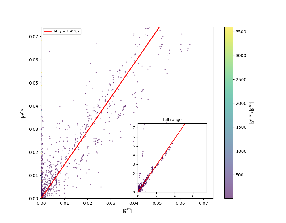
Computing the ZPR with GWPT e-ph matrix elements
In this section, we finally compute the ZPR of MgO at the GWPT level using the results produced previously. As you will see the calculation is much faster than the previous step as this run is essentially a post-processing of the data stored in the GSTORE file.
The price to pay is that there are few parameters that can be changed as this level. In other words, the quality of the ZPR obtained here mainly depends on the density of the \(\qq\)- and \(\pp\)-meshes used in the previous section, the number of empty states (\(n'\) index) and the different cutoff energies.
In order to perform convergence studies, one should go back to the previous step, increase the relevant parameters and monitor how the ZPR is affected by these settings. Let us stress again that the calculations in this tutorial are severely underconverged and there are several theoretical and technical and aspect that are still under investigation.
After this preamble, let us start the calculation by issuing:
mpirun -n 4 abinit teph4zpr_gwpt_8.abi > teph4zpr_8.log 2> err &
with the following input file:
# Computation of ZPR from GSTORE file with GWPT matrix elements.

ngkpt 4 4 4
nshiftk 1
shiftk 0 0 0

optdriver 7   # Enter EPH driver.
eph_task 24   # ZPR from GSTORE.
getgstore_filepath "teph4zpr_gwpt_7o_GSTORE.nc"

tmesh 0 100 4             # [start, step, num_T] in Kelvin

nband 20
eph_stern 1              # Activate Sterheimer method
gwpt_g2mode 2            # See documentation.
zcut 0.01 eV             # Imaginary shift in Green's function denominator.
#gstore_gname "gvals_ks" # Activate this line to use KS matrix elements

ddb_ngqpt 4 4 4

getwfk_filepath "teph4zpr_gwpt_4o_WFK"    # 4x4x4 k-mesh
getpot_filepath "MgO_eph_zpr/flow_zpr_mgo/w0/t0/outdata/out_POT.nc"
getddb_filepath "teph4zpr_gwpt_1_DDB"
getdvdb_filepath "teph4zpr_gwpt_2_DVDB"

ecut 35.0

prtphdos 0       # Disable computation of PHDOS to save some time

pp_dirpath = "$ABI_PSPDIR"
pseudos = "O.psp8, Mg-sp-gw.psp8"

structure = "abifile:MgO_eph_zpr/flow_zpr_mgo/w0/t0/outdata/out_DEN.nc"

##############################################################
# This section is used only for regression testing of ABINIT #
##############################################################
#%%<BEGIN TEST_INFO>
#%% [setup]
#%% executable = abinit
#%% test_chain =  teph4zpr_gwpt_1.abi, teph4zpr_gwpt_2.abi, teph4zpr_gwpt_3.abi, teph4zpr_gwpt_4.abi,
#%%               teph4zpr_gwpt_5.abi, teph4zpr_gwpt_6.abi, teph4zpr_gwpt_7.abi, teph4zpr_gwpt_8.abi
#%% exclude_builders = scope_gnu_10.2_paral
#%% [files]
#%% use_git_submodule = MgO_eph_zpr
#%% files_to_test =
#%%   teph4zpr_gwpt_8.abo, tolnlines= 57, tolabs=  3.000e-02, tolrel=  6.000e-03
#%% [paral_info]
#%% max_nprocs = 10
#%% [extra_info]
#%% authors = M. Giantomassi
#%% keywords = NC, DFPT, EPH, GWPT
#%% description = Computation of ZPR from GSTORE file with GWPT matrix elements.
#%%<END TEST_INFO>
Let us now discuss the most relevant input variables:
To activate the computation of the e-ph self-energy from a GSTORE file we use optdriver, eph_task and getgstore_filepath
optdriver 7   # Enter EPH driver.
eph_task 24   # ZPR from GSTORE.
getgstore_filepath "teph4zpr_gwpt_7o_GSTORE.nc"
The temperature mesh in Kelvin is defined by tmesh. The imaginary shift in the denominator of the self-energy is given by zcut.
We also use eph_stern 1 and getpot_filepath to activate the Sternheimer approach to account for the contribution of the bands beyond the active space defined by nband.
Important
The Sternheimer method is exact if one is interested in the on-the-mass-shell corrections at the KS level in the adiabatic approximation. In the case of GWPT calculations, one assumes that the GWPT matrix elements are very close to the KS ones when \(m\) > nband.
Now let us have a look at the final results reported in the main output file:
.Version 10.7.2.6 of ABINIT. v10.7.1 released Mar 2026.
.(MPI version, prepared for a aarch64_darwin23.6.0_gnu14.2 computer)
.Copyright (C) 1998-2025 ABINIT group .
ABINIT comes with ABSOLUTELY NO WARRANTY.
It is free software, and you are welcome to redistribute it
under certain conditions (GNU General Public License,
see ~abinit/COPYING or http://www.gnu.org/copyleft/gpl.txt).
ABINIT is a project of the Universite Catholique de Louvain,
Corning Inc. and other collaborators, see ~abinit/doc/developers/contributors.txt .
Please read https://docs.abinit.org/theory/acknowledgments for suggested
acknowledgments of the ABINIT effort.
For more information, see https://www.abinit.org .
.Starting date : Thu 20 Nov 2025.
- ( at 04h26 )
- input file -> /Users/giantomassi/git_repos/abinit/_build/tests/Test_suite/tutorespfn_teph4zpr_gwpt_1-teph4zpr_gwpt_2-teph4zpr_gwpt_3-teph4zpr_gwpt_4-teph4zpr_gwpt_5-teph4zpr_gwpt_6-teph4zpr_gwpt_7-teph4zpr_gwpt_8/teph4zpr_gwpt_8.abi
- output file -> teph4zpr_gwpt_8.abo
- root for input files -> teph4zpr_gwpt_8i
- root for output files -> teph4zpr_gwpt_8o
Symmetries : space group Fm -3 m (#225); Bravais cF (face-center cubic)
================================================================================
Values of the parameters that define the memory need of the present run
intxc = 0 ionmov = 0 iscf = 7 lmnmax = 5
lnmax = 5 mgfft = 32 mpssoang = 3 mqgrid = 3001
natom = 2 nloc_mem = 1 nspden = 1 nspinor = 1
nsppol = 1 nsym = 48 n1xccc = 2501 ntypat = 2
occopt = 1 xclevel = 2
- mband = 20 mffmem = 1 mkmem = 8
mpw = 1304 nfft = 32768 nkpt = 8
================================================================================
P This job should need less than 14.907 Mbytes of memory.
Rough estimation (10% accuracy) of disk space for files :
_ WF disk file : 3.186 Mbytes ; DEN or POT disk file : 0.252 Mbytes.
================================================================================
--------------------------------------------------------------------------------
------------- Echo of variables that govern the present computation ------------
--------------------------------------------------------------------------------
-
- outvars: echo of selected default values
- iomode0 = 0 , fftalg0 =312 , wfoptalg0 = 0
-
- outvars: echo of global parameters not present in the input file
- max_nthreads = 0
-
-outvars: echo values of preprocessed input variables --------
acell 1.0000000000E+00 1.0000000000E+00 1.0000000000E+00 Bohr
amu 1.59994000E+01 2.43050000E+01
ddb_ngqpt 4 4 4
ecut 3.50000000E+01 Hartree
eph_stern 1
eph_task 24
- fftalg 312
gwpt_g2mode 2
istwfk 2 0 3 0 0 0 7 0
ixc 11
kpt 0.00000000E+00 0.00000000E+00 0.00000000E+00
2.50000000E-01 0.00000000E+00 0.00000000E+00
5.00000000E-01 0.00000000E+00 0.00000000E+00
2.50000000E-01 2.50000000E-01 0.00000000E+00
5.00000000E-01 2.50000000E-01 0.00000000E+00
-2.50000000E-01 2.50000000E-01 0.00000000E+00
5.00000000E-01 5.00000000E-01 0.00000000E+00
-2.50000000E-01 5.00000000E-01 2.50000000E-01
kptrlatt 4 0 0 0 4 0 0 0 4
kptrlen 2.27305763E+01
P mkmem 8
natom 2
nband 20
ngfft 32 32 32
nkpt 8
nline 100
nsym 48
ntypat 2
occ 2.000000 2.000000 2.000000 2.000000 2.000000 2.000000
2.000000 2.000000 0.000000 0.000000 0.000000 0.000000
0.000000 0.000000 0.000000 0.000000 0.000000 0.000000
0.000000 0.000000
optdriver 7
prtphdos 0
rprim 0.0000000000E+00 4.0182361526E+00 4.0182361526E+00
4.0182361526E+00 0.0000000000E+00 4.0182361526E+00
4.0182361526E+00 4.0182361526E+00 0.0000000000E+00
spgroup 225
symrel 1 0 0 0 1 0 0 0 1 -1 0 0 0 -1 0 0 0 -1
0 -1 1 0 -1 0 1 -1 0 0 1 -1 0 1 0 -1 1 0
-1 0 0 -1 0 1 -1 1 0 1 0 0 1 0 -1 1 -1 0
0 1 -1 1 0 -1 0 0 -1 0 -1 1 -1 0 1 0 0 1
-1 0 0 -1 1 0 -1 0 1 1 0 0 1 -1 0 1 0 -1
0 -1 1 1 -1 0 0 -1 0 0 1 -1 -1 1 0 0 1 0
1 0 0 0 0 1 0 1 0 -1 0 0 0 0 -1 0 -1 0
0 1 -1 0 0 -1 1 0 -1 0 -1 1 0 0 1 -1 0 1
-1 0 1 -1 1 0 -1 0 0 1 0 -1 1 -1 0 1 0 0
0 -1 0 1 -1 0 0 -1 1 0 1 0 -1 1 0 0 1 -1
1 0 -1 0 0 -1 0 1 -1 -1 0 1 0 0 1 0 -1 1
0 1 0 0 0 1 1 0 0 0 -1 0 0 0 -1 -1 0 0
1 0 -1 0 1 -1 0 0 -1 -1 0 1 0 -1 1 0 0 1
0 -1 0 0 -1 1 1 -1 0 0 1 0 0 1 -1 -1 1 0
-1 0 1 -1 0 0 -1 1 0 1 0 -1 1 0 0 1 -1 0
0 1 0 1 0 0 0 0 1 0 -1 0 -1 0 0 0 0 -1
0 0 -1 0 1 -1 1 0 -1 0 0 1 0 -1 1 -1 0 1
1 -1 0 0 -1 1 0 -1 0 -1 1 0 0 1 -1 0 1 0
0 0 1 1 0 0 0 1 0 0 0 -1 -1 0 0 0 -1 0
-1 1 0 -1 0 0 -1 0 1 1 -1 0 1 0 0 1 0 -1
0 0 1 0 1 0 1 0 0 0 0 -1 0 -1 0 -1 0 0
1 -1 0 0 -1 0 0 -1 1 -1 1 0 0 1 0 0 1 -1
0 0 -1 1 0 -1 0 1 -1 0 0 1 -1 0 1 0 -1 1
-1 1 0 -1 0 1 -1 0 0 1 -1 0 1 0 -1 1 0 0
tolwfr 1.00000000E-16
tmesh 0.00000000E+00 1.00000000E+02 4.00000000E+00
typat 2 1
wtk 0.01563 0.12500 0.06250 0.09375 0.37500 0.18750
0.04688 0.09375
xangst 0.0000000000E+00 0.0000000000E+00 0.0000000000E+00
2.1263589985E+00 2.1263589985E+00 2.1263589985E+00
xcart 0.0000000000E+00 0.0000000000E+00 0.0000000000E+00
4.0182361526E+00 4.0182361526E+00 4.0182361526E+00
xred 0.0000000000E+00 0.0000000000E+00 0.0000000000E+00
5.0000000000E-01 5.0000000000E-01 5.0000000000E-01
zcut 3.67493222E-04 Hartree
znucl 8.00000 12.00000
================================================================================
chkinp: Checking input parameters for consistency.
================================================================================
== DATASET 1 ==================================================================
- mpi_nproc: 1, omp_nthreads: -1 (-1 if OMP is not activated)
--- !DatasetInfo
iteration_state: {dtset: 1, }
dimensions: {natom: 2, nkpt: 8, mband: 20, nsppol: 1, nspinor: 1, nspden: 1, mpw: 1304, }
cutoff_energies: {ecut: 35.0, pawecutdg: -1.0, }
electrons: {nelect: 1.60000000E+01, charge: 0.00000000E+00, occopt: 1.00000000E+00, tsmear: 1.00000000E-02, }
meta: {optdriver: 7, eph_task: 24, }
...
mkfilename: getwfk from: teph4zpr_gwpt_4o_WFK
mkfilename: getddb from: teph4zpr_gwpt_1_DDB
mkfilename: getpot from: MgO_eph_zpr/flow_zpr_mgo/w0/t0/outdata/out_POT.nc
mkfilename: getdvdb from: teph4zpr_gwpt_2_DVDB
mkfilename: getgstore from: teph4zpr_gwpt_7o_GSTORE.nc
Exchange-correlation functional for the present dataset will be:
GGA: Perdew-Burke-Ernzerhof functional - ixc=11
Citation for XC functional:
J.P.Perdew, K.Burke, M.Ernzerhof, PRL 77, 3865 (1996)
- Reading GS states from WFK file: teph4zpr_gwpt_4o_WFK
- Reading DDB from file: teph4zpr_gwpt_1_DDB
- Reading DVDB from file: teph4zpr_gwpt_2_DVDB
==== Info on the Cryst% object ====
Real(R)+Recip(G) space primitive vectors, cartesian coordinates (Bohr,Bohr^-1):
R(1)= 0.0000000 4.0182362 4.0182362 G(1)= -0.1244327 0.1244327 0.1244327
R(2)= 4.0182362 0.0000000 4.0182362 G(2)= 0.1244327 -0.1244327 0.1244327
R(3)= 4.0182362 4.0182362 0.0000000 G(3)= 0.1244327 0.1244327 -0.1244327
Unit cell volume ucvol= 1.2975866E+02 bohr^3
Angles (23,13,12)= 6.00000000E+01 6.00000000E+01 6.00000000E+01 degrees
Time-reversal symmetry is present
Reduced atomic positions [iatom, xred, symbol]:
1) 0.0000000 0.0000000 0.0000000 Mg
2) 0.5000000 0.5000000 0.5000000 O
DDB file with 8 blocks has been read.
================================================================================
Dielectric Tensor and Effective Charges
anaddb : Zero the imaginary part of the Dynamical Matrix at Gamma,
and impose the ASR on the effective charges
The violation of the charge neutrality conditions
by the effective charges is as follows :
atom electric field
displacement direction
1 1 -0.085945 0.000000
1 2 0.000000 0.000000
1 3 0.000000 0.000000
2 1 0.000000 0.000000
2 2 -0.085945 0.000000
2 3 -0.000000 0.000000
3 1 -0.000000 0.000000
3 2 -0.000000 0.000000
3 3 -0.085945 0.000000
Effective charge tensors after
imposition of the charge neutrality (if requested by user),
and eventual restriction to some part :
atom displacement
1 1 2.040887E+00 -1.659033E-16 -1.658285E-16
1 2 -1.659033E-16 2.040887E+00 1.659781E-16
1 3 1.659033E-16 1.659033E-16 2.040887E+00
2 1 -2.040887E+00 1.659033E-16 1.658285E-16
2 2 1.659033E-16 -2.040887E+00 -1.659781E-16
2 3 -1.659033E-16 -1.659033E-16 -2.040887E+00
Now, the imaginary part of the dynamical matrix is zeroed
- Found dielectric tensor and Born effective charges in DDB file: teph4zpr_gwpt_1_DDB
- Cannot find quadrupole tensor in DDB file: teph4zpr_gwpt_1_DDB
Values initialized with zeros.
Homogeneous q point set in the B.Z.
Grid q points : 64
1) 0.00000000E+00 0.00000000E+00 0.00000000E+00
2) 2.50000000E-01 0.00000000E+00 0.00000000E+00
3) 5.00000000E-01 0.00000000E+00 0.00000000E+00
4) -2.50000000E-01 0.00000000E+00 0.00000000E+00
5) 0.00000000E+00 2.50000000E-01 0.00000000E+00
6) 2.50000000E-01 2.50000000E-01 0.00000000E+00
7) 5.00000000E-01 2.50000000E-01 0.00000000E+00
8) -2.50000000E-01 2.50000000E-01 0.00000000E+00
9) 0.00000000E+00 5.00000000E-01 0.00000000E+00
10) 2.50000000E-01 5.00000000E-01 0.00000000E+00
11) 5.00000000E-01 5.00000000E-01 0.00000000E+00
12) -2.50000000E-01 5.00000000E-01 0.00000000E+00
13) 0.00000000E+00 -2.50000000E-01 0.00000000E+00
14) 2.50000000E-01 -2.50000000E-01 0.00000000E+00
15) 5.00000000E-01 -2.50000000E-01 0.00000000E+00
16) -2.50000000E-01 -2.50000000E-01 0.00000000E+00
17) 0.00000000E+00 0.00000000E+00 2.50000000E-01
18) 2.50000000E-01 0.00000000E+00 2.50000000E-01
19) 5.00000000E-01 0.00000000E+00 2.50000000E-01
20) -2.50000000E-01 0.00000000E+00 2.50000000E-01
21) 0.00000000E+00 2.50000000E-01 2.50000000E-01
22) 2.50000000E-01 2.50000000E-01 2.50000000E-01
23) 5.00000000E-01 2.50000000E-01 2.50000000E-01
24) -2.50000000E-01 2.50000000E-01 2.50000000E-01
25) 0.00000000E+00 5.00000000E-01 2.50000000E-01
26) 2.50000000E-01 5.00000000E-01 2.50000000E-01
27) 5.00000000E-01 5.00000000E-01 2.50000000E-01
28) -2.50000000E-01 5.00000000E-01 2.50000000E-01
29) 0.00000000E+00 -2.50000000E-01 2.50000000E-01
30) 2.50000000E-01 -2.50000000E-01 2.50000000E-01
31) 5.00000000E-01 -2.50000000E-01 2.50000000E-01
32) -2.50000000E-01 -2.50000000E-01 2.50000000E-01
33) 0.00000000E+00 0.00000000E+00 5.00000000E-01
34) 2.50000000E-01 0.00000000E+00 5.00000000E-01
35) 5.00000000E-01 0.00000000E+00 5.00000000E-01
36) -2.50000000E-01 0.00000000E+00 5.00000000E-01
37) 0.00000000E+00 2.50000000E-01 5.00000000E-01
38) 2.50000000E-01 2.50000000E-01 5.00000000E-01
39) 5.00000000E-01 2.50000000E-01 5.00000000E-01
40) -2.50000000E-01 2.50000000E-01 5.00000000E-01
41) 0.00000000E+00 5.00000000E-01 5.00000000E-01
42) 2.50000000E-01 5.00000000E-01 5.00000000E-01
43) 5.00000000E-01 5.00000000E-01 5.00000000E-01
44) -2.50000000E-01 5.00000000E-01 5.00000000E-01
45) 0.00000000E+00 -2.50000000E-01 5.00000000E-01
46) 2.50000000E-01 -2.50000000E-01 5.00000000E-01
47) 5.00000000E-01 -2.50000000E-01 5.00000000E-01
48) -2.50000000E-01 -2.50000000E-01 5.00000000E-01
49) 0.00000000E+00 0.00000000E+00 -2.50000000E-01
50) 2.50000000E-01 0.00000000E+00 -2.50000000E-01
51) 5.00000000E-01 0.00000000E+00 -2.50000000E-01
52) -2.50000000E-01 0.00000000E+00 -2.50000000E-01
53) 0.00000000E+00 2.50000000E-01 -2.50000000E-01
54) 2.50000000E-01 2.50000000E-01 -2.50000000E-01
55) 5.00000000E-01 2.50000000E-01 -2.50000000E-01
56) -2.50000000E-01 2.50000000E-01 -2.50000000E-01
57) 0.00000000E+00 5.00000000E-01 -2.50000000E-01
58) 2.50000000E-01 5.00000000E-01 -2.50000000E-01
59) 5.00000000E-01 5.00000000E-01 -2.50000000E-01
60) -2.50000000E-01 5.00000000E-01 -2.50000000E-01
61) 0.00000000E+00 -2.50000000E-01 -2.50000000E-01
62) 2.50000000E-01 -2.50000000E-01 -2.50000000E-01
63) 5.00000000E-01 -2.50000000E-01 -2.50000000E-01
64) -2.50000000E-01 -2.50000000E-01 -2.50000000E-01
The interatomic forces have been obtained
--- Pseudopotential description ------------------------------------------------
- pspini: atom type 1 psp file is /Users/giantomassi/git_repos/abinit/tests/Pspdir/O.psp8
- pspatm: opening atomic psp file /Users/giantomassi/git_repos/abinit/tests/Pspdir/O.psp8
- O ONCVPSP r_core= 1.36 1.46 1.26
- 8.00000 6.00000 151103 znucl, zion, pspdat
8 11 2 4 600 0.00000 pspcod,pspxc,lmax,lloc,mmax,r2well
5.99000000000000 4.00000000000000 0.00000000000000 rchrg,fchrg,qchrg
nproj 2 2 1
extension_switch 1
pspatm : epsatm= 6.19401560
--- l ekb(1:nproj) -->
0 5.257212 0.704241
1 -5.135443 -1.451781
2 -4.371486
pspatm: atomic psp has been read and splines computed
- pspini: atom type 2 psp file is /Users/giantomassi/git_repos/abinit/tests/Pspdir/Mg-sp-gw.psp8
- pspatm: opening atomic psp file /Users/giantomassi/git_repos/abinit/tests/Pspdir/Mg-sp-gw.psp8
- Mg ONCVPSP r_core= 1.16 1.56
- 12.00000 10.00000 150902 znucl, zion, pspdat
8 11 1 4 400 0.00000 pspcod,pspxc,lmax,lloc,mmax,r2well
3.99000000000000 0.00000000000000 0.00000000000000 rchrg,fchrg,qchrg
nproj 2 2
extension_switch 1
pspatm : epsatm= 9.22508734
--- l ekb(1:nproj) -->
0 2.568049 -0.805950
1 -6.605901 -2.664074
pspatm: atomic psp has been read and splines computed
2.46705647E+02 ecore*ucvol(ha*bohr**3)
--------------------------------------------------------------------------------
Computing Fan-Migdal + DW self-energy from GSTORE.nc
Using e-ph self-energy expression with g^*_KS g_GWPT
- Reading e-ph matrix elements from: teph4zpr_gwpt_7o_GSTORE.nc
Asking for with_cplex: 2
Asking for with_gmode: phonon
Asking for gvals_name: gvals
Asking for g2dw: yes
Initializing gstore object from: teph4zpr_gwpt_7o_GSTORE.nc
Reading GWPT e-ph matrix elements
P qpt_comm can use shmem: yes
P kpt_comm can use shmem: yes
P bsum_comm can use shmem: yes
P pp_sum_comm can use shmem: yes
=== Gstore parameters ===
kzone: ibz
kfilter: qprange
nkibz: 8
nkbz: 64
glob_nk_spin: [1]
qzone: bz
nqibz: 8
nqbz: 64
glob_nq_spin: [64]
kptopt: 1
qptopt: 1
has_used_lgk: 1
has_used_lgq: 0
with_vk: 1
gqk_cplex: 2
gqk_bstart_k: 6
gqk_bstart_kq: 1
gqk_bstop_k: 9
gqk_bstop_kq: 10
gqk_nb_k: 4
gqk_nb_kq: 10
gqk_my_npert: 6
P gqk_my_nk: -1
P gqk_my_nq: -1
=== MPI distribution ===
P Number of CPUs for parallelism over perturbations: 1
P Number of perturbations treated by this CPU: 6
P Number of CPUs for parallelism over q-points: 1
P Number of CPUs for parallelism over k-points: 1
k-points included in gstore:
1 : [ 0.0000E+00, 0.0000E+00, 0.0000E+00]
Little group operations of the k-point will be used to symmetry reduce the integral in q-space.
=== Gaps, band edges and relative position wrt Fermi level ===
Direct band gap semiconductor
Fundamental gap: 4.479 (eV)
VBM: 4.490 (eV) at k: [ 0.0000E+00, 0.0000E+00, 0.0000E+00]
CBM: 8.969 (eV) at k: [ 0.0000E+00, 0.0000E+00, 0.0000E+00]
Direct gap: 4.479 (eV) at k: [ 0.0000E+00, 0.0000E+00, 0.0000E+00]
Position of CBM/VBM with respect to the Fermi level:
Notations: mu_e = Fermi level, D_v = (mu_e - VBM), D_c = (CBM - mu_e)
T(K) kT (eV) mu_e (eV) D_v (eV) D_c (eV)
0.0 0.000 7.270 2.781 1.698
100.0 0.009 7.173 2.684 1.795
200.0 0.017 7.077 2.587 1.892
300.0 0.026 6.980 2.490 1.989
Reading GS KS potential for Sternheimer from: MgO_eph_zpr/flow_zpr_mgo/w0/t0/outdata/out_POT.nc
================================================================================
Final results in eV.
Notations:
eKS: Kohn-Sham energy. eQP: quasi-particle energy.
eQP - eKS: Difference between the QP and the KS energy.
SE1(eKS): Real part of the self-energy computed at the KS energy, SE2 for imaginary part.
Z(eKS): Renormalization factor.
FAN: Real part of the Fan term at eKS. DW: Debye-Waller term.
DeKS: KS energy difference between this band and band-1, DeQP same meaning but for eQP.
OTMS: On-the-mass-shell approximation with eQP ~= eKS + Sigma(omega=eKS)
TAU(eKS): Lifetime in femtoseconds computed at the KS energy.
mu_e: Fermi level for given (T, nelect)
Using g(k,q) of type: GWPT
K-point: [ 0.0000E+00, 0.0000E+00, 0.0000E+00], T: 0.0 [K], mu_e: 7.270
B eKS eQP eQP-eKS SE1(eKS) SE2(eKS) Z(eKS) FAN(eKS) DW DeKS DeQP
6 4.490 4.689 0.199 0.313 -0.006 0.637 -3.809 4.122 0.000 0.000
7 4.490 4.689 0.199 0.313 -0.006 0.637 -3.809 4.122 0.000 0.000
8 4.490 4.689 0.199 0.313 -0.006 0.637 -3.809 4.122 0.000 0.000
9 8.969 8.867 -0.102 -0.104 -0.000 0.979 0.035 -0.139 4.479 4.178
KS gap: 4.479 (assuming bval:8 ==> bcond:9)
QP gap: 4.178 (OTMS: 4.062)
QP_gap - KS_gap: -0.301 (OTMS: -0.417)
============================================================================================
K-point: [ 0.0000E+00, 0.0000E+00, 0.0000E+00], T: 100.0 [K], mu_e: 7.173
B eKS eQP eQP-eKS SE1(eKS) SE2(eKS) Z(eKS) FAN(eKS) DW DeKS DeQP
6 4.490 4.689 0.199 0.313 -0.006 0.637 -3.900 4.213 0.000 0.000
7 4.490 4.689 0.199 0.313 -0.006 0.637 -3.900 4.213 0.000 0.000
8 4.490 4.689 0.199 0.313 -0.006 0.637 -3.900 4.213 0.000 0.000
9 8.969 8.866 -0.103 -0.105 -0.000 0.979 0.043 -0.148 4.479 4.177
KS gap: 4.479 (assuming bval:8 ==> bcond:9)
QP gap: 4.177 (OTMS: 4.061)
QP_gap - KS_gap: -0.302 (OTMS: -0.418)
============================================================================================
K-point: [ 0.0000E+00, 0.0000E+00, 0.0000E+00], T: 200.0 [K], mu_e: 7.077
B eKS eQP eQP-eKS SE1(eKS) SE2(eKS) Z(eKS) FAN(eKS) DW DeKS DeQP
6 4.490 4.691 0.202 0.316 -0.006 0.639 -4.552 4.868 0.000 0.000
7 4.490 4.691 0.202 0.316 -0.006 0.639 -4.552 4.868 0.000 0.000
8 4.490 4.691 0.202 0.316 -0.006 0.639 -4.552 4.868 0.000 0.000
9 8.969 8.857 -0.112 -0.115 -0.000 0.975 0.082 -0.197 4.479 4.165
KS gap: 4.479 (assuming bval:8 ==> bcond:9)
QP gap: 4.165 (OTMS: 4.048)
QP_gap - KS_gap: -0.314 (OTMS: -0.431)
============================================================================================
K-point: [ 0.0000E+00, 0.0000E+00, 0.0000E+00], T: 300.0 [K], mu_e: 6.980
B eKS eQP eQP-eKS SE1(eKS) SE2(eKS) Z(eKS) FAN(eKS) DW DeKS DeQP
6 4.490 4.700 0.211 0.339 -0.006 0.621 -5.626 5.965 0.000 0.000
7 4.490 4.700 0.211 0.339 -0.006 0.621 -5.626 5.965 0.000 0.000
8 4.490 4.700 0.211 0.339 -0.006 0.621 -5.626 5.965 0.000 0.000
9 8.969 8.838 -0.131 -0.135 -0.000 0.970 0.128 -0.263 4.479 4.137
KS gap: 4.479 (assuming bval:8 ==> bcond:9)
QP gap: 4.137 (OTMS: 4.005)
QP_gap - KS_gap: -0.342 (OTMS: -0.474)
============================================================================================
== END DATASET(S) ==============================================================
================================================================================
-outvars: echo values of variables after computation --------
acell 1.0000000000E+00 1.0000000000E+00 1.0000000000E+00 Bohr
amu 1.59994000E+01 2.43050000E+01
ddb_ngqpt 4 4 4
ecut 3.50000000E+01 Hartree
eph_stern 1
eph_task 24
etotal 0.0000000000E+00
fcart 0.0000000000E+00 0.0000000000E+00 0.0000000000E+00
0.0000000000E+00 0.0000000000E+00 0.0000000000E+00
- fftalg 312
gwpt_g2mode 2
ixc 11
kptrlatt 4 0 0 0 4 0 0 0 4
kptrlen 2.27305763E+01
P mkmem 8
natom 2
nband 20
ngfft 32 32 32
nkpt 8
nline 100
nsym 48
ntypat 2
occ 2.000000 2.000000 2.000000 2.000000 2.000000 2.000000
2.000000 2.000000 0.000000 0.000000 0.000000 0.000000
0.000000 0.000000 0.000000 0.000000 0.000000 0.000000
0.000000 0.000000
optdriver 7
prtphdos 0
rprim 0.0000000000E+00 4.0182361526E+00 4.0182361526E+00
4.0182361526E+00 0.0000000000E+00 4.0182361526E+00
4.0182361526E+00 4.0182361526E+00 0.0000000000E+00
spgroup 225
strten 0.0000000000E+00 0.0000000000E+00 0.0000000000E+00
0.0000000000E+00 0.0000000000E+00 0.0000000000E+00
symrel 1 0 0 0 1 0 0 0 1 -1 0 0 0 -1 0 0 0 -1
0 -1 1 0 -1 0 1 -1 0 0 1 -1 0 1 0 -1 1 0
-1 0 0 -1 0 1 -1 1 0 1 0 0 1 0 -1 1 -1 0
0 1 -1 1 0 -1 0 0 -1 0 -1 1 -1 0 1 0 0 1
-1 0 0 -1 1 0 -1 0 1 1 0 0 1 -1 0 1 0 -1
0 -1 1 1 -1 0 0 -1 0 0 1 -1 -1 1 0 0 1 0
1 0 0 0 0 1 0 1 0 -1 0 0 0 0 -1 0 -1 0
0 1 -1 0 0 -1 1 0 -1 0 -1 1 0 0 1 -1 0 1
-1 0 1 -1 1 0 -1 0 0 1 0 -1 1 -1 0 1 0 0
0 -1 0 1 -1 0 0 -1 1 0 1 0 -1 1 0 0 1 -1
1 0 -1 0 0 -1 0 1 -1 -1 0 1 0 0 1 0 -1 1
0 1 0 0 0 1 1 0 0 0 -1 0 0 0 -1 -1 0 0
1 0 -1 0 1 -1 0 0 -1 -1 0 1 0 -1 1 0 0 1
0 -1 0 0 -1 1 1 -1 0 0 1 0 0 1 -1 -1 1 0
-1 0 1 -1 0 0 -1 1 0 1 0 -1 1 0 0 1 -1 0
0 1 0 1 0 0 0 0 1 0 -1 0 -1 0 0 0 0 -1
0 0 -1 0 1 -1 1 0 -1 0 0 1 0 -1 1 -1 0 1
1 -1 0 0 -1 1 0 -1 0 -1 1 0 0 1 -1 0 1 0
0 0 1 1 0 0 0 1 0 0 0 -1 -1 0 0 0 -1 0
-1 1 0 -1 0 0 -1 0 1 1 -1 0 1 0 0 1 0 -1
0 0 1 0 1 0 1 0 0 0 0 -1 0 -1 0 -1 0 0
1 -1 0 0 -1 0 0 -1 1 -1 1 0 0 1 0 0 1 -1
0 0 -1 1 0 -1 0 1 -1 0 0 1 -1 0 1 0 -1 1
-1 1 0 -1 0 1 -1 0 0 1 -1 0 1 0 -1 1 0 0
tolwfr 1.00000000E-16
tmesh 0.00000000E+00 1.00000000E+02 4.00000000E+00
typat 2 1
xangst 0.0000000000E+00 0.0000000000E+00 0.0000000000E+00
2.1263589985E+00 2.1263589985E+00 2.1263589985E+00
xcart 0.0000000000E+00 0.0000000000E+00 0.0000000000E+00
4.0182361526E+00 4.0182361526E+00 4.0182361526E+00
xred 0.0000000000E+00 0.0000000000E+00 0.0000000000E+00
5.0000000000E-01 5.0000000000E-01 5.0000000000E-01
zcut 3.67493222E-04 Hartree
znucl 8.00000 12.00000
================================================================================
- Timing analysis has been suppressed with timopt=0
================================================================================
Suggested references for the acknowledgment of ABINIT usage.
The users of ABINIT have little formal obligations with respect to the ABINIT group
(those specified in the GNU General Public License, http://www.gnu.org/copyleft/gpl.txt).
However, it is common practice in the scientific literature,
to acknowledge the efforts of people that have made the research possible.
In this spirit, please find below suggested citations of work written by ABINIT developers,
corresponding to implementations inside of ABINIT that you have used in the present run.
Note also that it will be of great value to readers of publications presenting these results,
to read papers enabling them to understand the theoretical formalism and details
of the ABINIT implementation.
For information on why they are suggested, see also https://docs.abinit.org/theory/acknowledgments.
-
- [1] Abinit 2025: New Capabilities for the Predictive Modeling of Solids and Nanomaterials.
- J. Chem. Phys. 163, 164126 (2025).
- M.J. Verstraete, J. Abreu, G. Allemand, B. Amadon, G. Antonius,
- M. Azizi, L. Baguet, C. Barat, L. Bastogne, R. Bejaud, J.-M. Beuken,
- J. Bieder, A. Blanchet, F. Bottin, J. Bouchet, J. Bouquiaux, E. Bousquet,
- J. Boust, F. Brieuc, V. Brousseau-Couture, N. Brouwer, F. Bruneval,
- A. Castellano, E. Castiel, J.-B. Charraud, J. Clerouin, M. Cote, C. Duval,
- A. Gallo, F. Gendron, G. Geneste, Ph. Ghosez, M. Giantomassi, O. Gingras,
- F. Gomez-Ortiz, X. Gonze, F. Goudreault, A. Gruneis, R. Gupta, B. Guster,
- D.R. Hamann, Xu He, O. Hellman, N. Holzwarth, F. Jollet, P. Kestener,
- I.-M. Lygatsika, O. Nadeau, L. MacEnulty, E. Mara
- Comment: the sixth generic paper describing the ABINIT project.
- Note that a version of this paper, that is not formatted for J. Chem. Phys.
- is available at
- https://github.com/abinit/abinit_assets/tree/main/abinit_package/papers/ABINIT25.pdf .
- The licence allows the authors to put it on the Web.
- DOI and bibtex: see https://docs.abinit.org/theory/bibliography/#verstraete2025
-
- [2] Optimized norm-conserving Vanderbilt pseudopotentials.
- D.R. Hamann, Phys. Rev. B 88, 085117 (2013).
- Comment: Some pseudopotential generated using the ONCVPSP code were used.
- DOI and bibtex: see https://docs.abinit.org/theory/bibliography/#hamann2013
-
- [3] The Abinit project: Impact, environment and recent developments.
- Computer Phys. Comm. 248, 107042 (2020).
- X.Gonze, B. Amadon, G. Antonius, F.Arnardi, L.Baguet, J.-M.Beuken,
- J.Bieder, F.Bottin, J.Bouchet, E.Bousquet, N.Brouwer, F.Bruneval,
- G.Brunin, T.Cavignac, J.-B. Charraud, Wei Chen, M.Cote, S.Cottenier,
- J.Denier, G.Geneste, Ph.Ghosez, M.Giantomassi, Y.Gillet, O.Gingras,
- D.R.Hamann, G.Hautier, Xu He, N.Helbig, N.Holzwarth, Y.Jia, F.Jollet,
- W.Lafargue-Dit-Hauret, K.Lejaeghere, M.A.L.Marques, A.Martin, C.Martins,
- H.P.C. Miranda, F.Naccarato, K. Persson, G.Petretto, V.Planes, Y.Pouillon,
- S.Prokhorenko, F.Ricci, G.-M.Rignanese, A.H.Romero, M.M.Schmitt, M.Torrent,
- M.J.van Setten, B.Van Troeye, M.J.Verstraete, G.Zerah and J.W.Zwanzig
- Comment: the fifth generic paper describing the ABINIT project.
- Note that a version of this paper, that is not formatted for Computer Phys. Comm.
- is available at
- https://github.com/abinit/abinit_assets/tree/main/abinit_package/papers/ABINIT20.pdf .
- The licence allows the authors to put it on the Web.
- DOI and bibtex: see https://docs.abinit.org/theory/bibliography/#gonze2020
-
- [4] The Abinit project: Impact, environment and recent developments.
- Computer Phys. Comm. 248, 107042 (2020).
- X.Gonze, B. Amadon, G. Antonius, F.Arnardi, L.Baguet, J.-M.Beuken,
- J.Bieder, F.Bottin, J.Bouchet, E.Bousquet, N.Brouwer, F.Bruneval,
- G.Brunin, T.Cavignac, J.-B. Charraud, Wei Chen, M.Cote, S.Cottenier,
- J.Denier, G.Geneste, Ph.Ghosez, M.Giantomassi, Y.Gillet, O.Gingras,
- D.R.Hamann, G.Hautier, Xu He, N.Helbig, N.Holzwarth, Y.Jia, F.Jollet,
- W.Lafargue-Dit-Hauret, K.Lejaeghere, M.A.L.Marques, A.Martin, C.Martins,
- H.P.C. Miranda, F.Naccarato, K. Persson, G.Petretto, V.Planes, Y.Pouillon,
- S.Prokhorenko, F.Ricci, G.-M.Rignanese, A.H.Romero, M.M.Schmitt, M.Torrent,
- M.J.van Setten, B.Van Troeye, M.J.Verstraete, G.Zerah and J.W.Zwanzig
- Comment: a global overview of ABINIT, with focus on selected capabilities .
- Note that a version of this paper, that is not formatted for J. Chem. Phys.
- is available at
- https://github.com/abinit/abinit_assets/tree/main/abinit_package/papers/ABINIT20_JPC.pdf .
- The licence allows the authors to put it on the Web.
- DOI and bibtex: see https://docs.abinit.org/theory/bibliography/#romero2020
-
- [5] Recent developments in the ABINIT software package.
- Computer Phys. Comm. 205, 106 (2016).
- X.Gonze, F.Jollet, F.Abreu Araujo, D.Adams, B.Amadon, T.Applencourt,
- C.Audouze, J.-M.Beuken, J.Bieder, A.Bokhanchuk, E.Bousquet, F.Bruneval
- D.Caliste, M.Cote, F.Dahm, F.Da Pieve, M.Delaveau, M.Di Gennaro,
- B.Dorado, C.Espejo, G.Geneste, L.Genovese, A.Gerossier, M.Giantomassi,
- Y.Gillet, D.R.Hamann, L.He, G.Jomard, J.Laflamme Janssen, S.Le Roux,
- A.Levitt, A.Lherbier, F.Liu, I.Lukacevic, A.Martin, C.Martins,
- M.J.T.Oliveira, S.Ponce, Y.Pouillon, T.Rangel, G.-M.Rignanese,
- A.H.Romero, B.Rousseau, O.Rubel, A.A.Shukri, M.Stankovski, M.Torrent,
- M.J.Van Setten, B.Van Troeye, M.J.Verstraete, D.Waroquier, J.Wiktor,
- B.Xu, A.Zhou, J.W.Zwanziger.
- Comment: the fourth generic paper describing the ABINIT project.
- Note that a version of this paper, that is not formatted for Computer Phys. Comm.
- is available at
- https://github.com/abinit/abinit_assets/tree/main/abinit_package/papers/ABINIT16.pdf .
- The licence allows the authors to put it on the Web.
- DOI and bibtex: see https://docs.abinit.org/theory/bibliography/#gonze2016
-
- Proc. 0 individual time (sec): cpu= 3.4 wall= 3.4
================================================================================
Calculation completed.
.Delivered 0 WARNINGs and 5 COMMENTs to log file.
+Overall time at end (sec) : cpu= 6.7 wall= 6.7
- [ALL OK] MEMORY CONSUMPTION REPORT FOR C CODE:
- There were 64 allocations and 64 deallocations in C code
- [ALL OK] MEMORY CONSUMPTION REPORT FOR FORTRAN CODE:
- There were 2178799 allocations and 2178799 deallocations in Fortran
- Remaining memory at the end of the calculation is 0
 Computing Fan-Migdal + DW self-energy from GSTORE.nc
 Using e-ph self-energy expression with g^*_KS g_GWPT

- Reading e-ph matrix elements from: teph4zpr_gwpt_7o_GSTORE.nc
 Asking for with_cplex: 2
 Asking for with_gmode: phonon
 Asking for gvals_name: gvals
 Asking for g2dw: yes
 Initializing gstore object from: teph4zpr_gwpt_7o_GSTORE.nc

 Reading GWPT e-ph matrix elements
After this section, we have a summary of the GSTORE parameters:
 === Gstore parameters ===
 kzone: ibz
 kfilter: qprange
 nkibz: 8
 nkbz: 64
 glob_nk_spin: [1]
 qzone: bz
 nqibz: 8
 nqbz: 64
 glob_nq_spin: [64]
 kptopt: 1
 qptopt: 1
 has_used_lgk: 1
 has_used_lgq: 0
 with_vk: 1

 gqk_cplex: 2
 gqk_bstart_k: 6
 gqk_bstart_kq: 1
 gqk_bstop_k: 9
 gqk_bstop_kq: 10
 gqk_nb_k: 4
 gqk_nb_kq: 10
 gqk_my_npert: 6
P gqk_my_nk: -1
P gqk_my_nq: -1
As expected, we have only \(\kk\)-point in the e-ph matrix elements.
Then we find a section describing how the workload and memory is distributed across the MPI grid:
  === MPI distribution ===
P Number of CPUs for parallelism over perturbations: 1
P Number of perturbations treated by this CPU: 6
P Number of CPUs for parallelism over q-points: 1
P Number of CPUs for parallelism over k-points: 1
 k-points included in gstore:
1 : [ 0.0000E+00,  0.0000E+00,  0.0000E+00]
 Little group operations of the k-point will be used to symmetry reduce the integral in q-space.
 === Gaps, band edges and relative position wrt Fermi level ===
 Direct band gap semiconductor
 Fundamental gap:     4.479 (eV)
   VBM:     4.490 (eV) at k: [ 0.0000E+00,  0.0000E+00,  0.0000E+00]
   CBM:     8.969 (eV) at k: [ 0.0000E+00,  0.0000E+00,  0.0000E+00]
 Direct gap:         4.479 (eV) at k: [ 0.0000E+00,  0.0000E+00,  0.0000E+00]

 Position of CBM/VBM with respect to the Fermi level:
 Notations: mu_e = Fermi level, D_v = (mu_e - VBM), D_c = (CBM - mu_e)

  T(K)   kT (eV)  mu_e (eV)  D_v (eV)   D_c (eV)
   0.0     0.000     7.270     2.781     1.698
 100.0     0.009     7.173     2.684     1.795
 200.0     0.017     7.077     2.587     1.892
 300.0     0.026     6.980     2.490     1.989
The final results are summarized in this table:
 Final results in eV.
 Notations:
     eKS: Kohn-Sham energy. eQP: quasi-particle energy.
     eQP - eKS: Difference between the QP and the KS energy.
     SE1(eKS): Real part of the self-energy computed at the KS energy, SE2 for imaginary part.
     Z(eKS): Renormalization factor.
     FAN: Real part of the Fan term at eKS. DW: Debye-Waller term.
     DeKS: KS energy difference between this band and band-1, DeQP same meaning but for eQP.
     OTMS: On-the-mass-shell approximation with eQP ~= eKS + Sigma(omega=eKS)
     TAU(eKS): Lifetime in femtoseconds computed at the KS energy.
     mu_e: Fermi level for given (T, nelect)


 Using g(k,q) of type: GWPT


K-point: [ 0.0000E+00,  0.0000E+00,  0.0000E+00], T:    0.0 [K], mu_e:    7.270
   B    eKS     eQP    eQP-eKS   SE1(eKS)  SE2(eKS)  Z(eKS)  FAN(eKS)   DW      DeKS     DeQP
   6   4.490    4.689    0.199    0.313   -0.006    0.637   -3.809    4.122    0.000    0.000
   7   4.490    4.689    0.199    0.313   -0.006    0.637   -3.809    4.122    0.000    0.000
   8   4.490    4.689    0.199    0.313   -0.006    0.637   -3.809    4.122    0.000    0.000
   9   8.969    8.867   -0.102   -0.104   -0.000    0.979    0.035   -0.139    4.479    4.178

 KS gap:    4.479 (assuming bval:8 ==> bcond:9)
 QP gap:    4.178 (OTMS:    4.062)
 QP_gap - KS_gap:   -0.301 (OTMS:   -0.417)
In order to compute the ZPR with KS matrix elements, run the same input file but now use gstore_gname = “gvals_ks”. You should get:
 Using g(k,q) of type: KS


K-point: [ 0.0000E+00,  0.0000E+00,  0.0000E+00], T:    0.0 [K], mu_e:    7.270
   B    eKS     eQP    eQP-eKS   SE1(eKS)  SE2(eKS)  Z(eKS)  FAN(eKS)   DW      DeKS     DeQP
   6   4.490    4.570    0.080    0.097   -0.002    0.829   -4.014    4.111    0.000    0.000
   7   4.490    4.570    0.080    0.097   -0.002    0.829   -4.014    4.111    0.000    0.000
   8   4.490    4.570    0.080    0.097   -0.002    0.829   -4.014    4.111    0.000    0.000
   9   8.969    8.887   -0.081   -0.083   -0.000    0.983   -0.056   -0.027    4.479    4.317

 KS gap:    4.479 (assuming bval:8 ==> bcond:9)
 QP gap:    4.317 (OTMS:    4.299)
 QP_gap - KS_gap:   -0.162 (OTMS:   -0.180)
To summarize, with GWPT the on-the-mass-shell gap is 4.062 eV while KS gives 4.299. Again, these results should be carefully converged.
Tip
eph_ahc_type 0 can be used to use the adiabatic version of the Allen-Heine-Cardona equation. This is the version that should be used when comparing GWPT ZPR with finite-difference \(G_0 W_0\) calculations performed at fixed screening ignoring contributions beyond the rigid-ion approximation commonly used to deal with the Debye-Waller term.